Thesis by
Ravi Palanki
In Partial Fulfillment of the Requirements for the Degree of
Doctor of Philosophy
California Institute of Technology Pasadena, California
2004
c
2004
To
my parents
Acknowledgements
It takes a lot of good karma to have Prof. Robert McEliece as an adviser. His insightful thinking and his unbounded enthusiasm have always helped change his graduate students’ lives for the better, and I am no exception to this rule. I will always be indebted to him for guiding me through four of the most memorable years of my life.
My heartfelt thanks also go to Dr. Jonathan Yedidia for offering me internships at Mitsubishi Electric Research Laboratories and for being my mentor ever since. Working with him and Dr. Marc Fossorier of the University of Hawaii was a truly rewarding experience.
I would like to thank Profs. Michelle Effros, Babak Hassibi, P. P. Vaidyanathan and Dr. Sam Dolinar of JPL for agreeing to be on my candidacy or defense committees and for being excellent teachers. Much of my knowledge of communications and information theory comes from them.
I am grateful to Caltech’s administrative staff, especially Shirley Beatty, for their help in making my stay here extremely pleasant. I would also like to acknowledge gen-erous funding from the National Science Foundation, Qualcomm Corp., Sony Corp., the Lee Center for Advanced Networking and Mitsubishi Electric Research Labora-tories.
Abstract
The invention of turbo codes and low density parity check (LDPC) codes has made it possible for us for design error correcting codes with low decoding complexity and rates close to channel capacity. However, such codes have been studied in detail only for the most basic communication system, in which a single transmitter sends data to a single receiver over a channel whose statistics are known to both the transmitter and the receiver. Such a simplistic model is not valid in the case of a wireless network, where multiple transmitters might want to communicate with multiple receivers at the same time over a channel which can vary rapidly.
While the design of efficient error correction codes for a general wireless network is an extremely hard problem, it should be possible to design such codes for several important special cases. This thesis takes a few steps in that direction. We analyze the performance of low density parity check codes under iterative decoding in certain simple networks and prove Shannon-theoretic results for more complex networks.
Contents
Dedication iii
Acknowledgements iv
Abstract v
1 Introduction 1
1.1 Basics of channel coding . . . 3
1.1.1 Channel capacity . . . 3
1.1.2 Channel models . . . 4
1.1.3 Channel codes . . . 6
1.1.4 Capacity achieving codes . . . 7
1.2 Low density parity check codes . . . 8
1.2.1 Degree distributions . . . 9
1.2.2 Iterative decoding . . . 10
1.2.3 Capacity achieving distributions . . . 12
1.3 Thesis outline . . . 13
2 Rateless codes on noisy channels 16 2.1 Introduction . . . 16
2.2 Luby transform codes . . . 19
2.2.1 The robust soliton distribution . . . 20
2.3 LT codes on noisy channels . . . 21
2.3.1 Error floors . . . 22
2.5 Conclusion . . . 27
3 Graph-based codes for synchronous multiple access channels 28 3.1 Introduction to multiple access channels . . . 28
3.2 Decoding LDPC codes on a MAC . . . 29
3.3 The binary adder channel . . . 32
3.4 Design of LDPC codes for the BAC . . . 34
3.4.1 Density evolution on the BAC . . . 35
3.5 The noisy binary adder channel . . . 37
3.6 Conclusion . . . 40
4 Iterative decoding of multi-step majority logic decodable codes 42 4.1 Introduction . . . 42
4.2 A brief review of multi-step majority logic decodable codes . . . 43
4.3 Three-state decoding algorithm . . . 45
4.4 Decoding approaches . . . 47
4.4.1 Fixed cost approaches . . . 47
4.4.2 Variable cost approach . . . 49
4.5 Simulation results . . . 50
4.5.1 (255,127,21) EG code . . . 50
4.5.2 (511,256,31) EG (RM) code . . . 54
4.6 Extension to iterative decoding for the AWGN channel . . . 56
4.7 Conclusion . . . 57
5 On the capacity of wireless erasure relay networks 58 5.1 Introduction . . . 58
5.2 Model, definitions and main result . . . 60
5.2.2 Capacity . . . 61
5.3 Achievability . . . 62
5.3.1 Network operation . . . 62
5.3.2 Decoder . . . 63
5.3.3 Probability of error . . . 64
5.4 Converse . . . 69
5.5 Conclusion . . . 70
6 On the capacity achieving distributions of some vector channels 71 6.1 Introduction . . . 71
6.2 Mathematical background . . . 73
6.2.1 Kuhn-Tucker conditions . . . 73
6.2.2 Holomorphic functions . . . 75
6.3 The vector Gaussian channel . . . 77
6.4 The Rayleigh block fading channel . . . 79
6.5 General block fading channels . . . 84
6.6 Conclusion . . . 88
7 Conclusion 90
List of Figures
1.1 Canonical communication system model . . . 3
1.2 Tanner graph of (3,6)-regular LDPC code . . . 9
1.3 A general communication system . . . 14
2.1 The Tanner graphs of LDPC and LT codes . . . 20
2.2 Performance of LT codes generated using Luby’s distribution . . . 22
2.3 Performance of LT codes generated using sparse distribution . . . 24
2.4 Comparison of LT codes and raptor codes . . . 25
2.5 Performance of a raptor code on different channels . . . 26
2.6 Performance of a raptor code in a rateless setting . . . 27
3.1 LDPC codes on a MAC . . . 30
3.2 The graph-splitting technique . . . 35
3.3 Performance of graph-split codes . . . 36
3.4 Capacity region of the noisy BAC . . . 38
3.5 Performance of IRA codes on the noisy BAC . . . 39
4.1 BF decoding of the (255,127,21) EG code in low SNR regime . . . 50
4.2 BF decoding of the (255,127,21) EG code in high SNR regime . . . . 53
4.3 BF decoding of the (255,127,21) EG code for fixed number of errors . 53 4.4 BF decoding of the (511,256,31) EG (or RM) code . . . 54
Chapter 1
Introduction
Digital communications technology has had an unrivaled impact on society over the course of the last few decades. With applications ranging from sophisticated military satellites and NASA’s Mars Rovers to the ubiquitous Internet and cell phones used every day by billions of people, digital communications systems have altered almost every aspect of our lives. Yet, none of these systems would exist today were it not for Claude Shannon and his seminal paper, “The mathematical theory of communi-cation” [71].
In this paper, originally published in 1948, Shannon gave the first quantitative definition of information, thereby creating the field of information theory. Shannon also proved that reliable communication of information over inherently unreliable channels is feasible. This means that even though a transmitter sends a message over a channel that corrupts or destroys part of the transmitted signal, the receiver can figure out precisely what message was sent. This counter-intuitive result, known as the “channel coding theorem,” also tells us that such reliable communication is possible if and only if the information transmission rate R (measured in bits per channel use) is less than a threshold known as the “channel capacity”C (also measured in bits per channel use).
chan-nel. Even though these n bits are corrupted by the time they reach the receiver, the receiver can use the redundant bits to try to figure out (or “decode”) the original k
bits.
Shannon showed that as k → ∞, with a judicious choice of the channel code, the receiver can almost surely infer what the transmitter sent. Moreover, the rate of the codeR =4 k/ncan be made arbitrarily close to the channel capacityC. Unfortunately, Shannon’s choice for the channel code is impossible to implement in practical systems, because the computational complexity of the decoder is unacceptably high. This led to one of the most important problems in information theory viz., to find practical channel codes whose rates are close to the channel capacity.
This problem proved to be extremely hard to solve. Even though information theorists constructed a wide variety of practical channel codes, none of these codes had rates close to channel capacity. It was only in 1993 that Berrou, Glavieux and Thitimajshima [5] developed “turbo codes,” the first practical codes that had rates close to capacity. This breakthrough revolutionized the field of channel coding and led to the development of low density parity check (LDPC) codes [22, 45, 66], which are state-of-the-art codes that have near-capacity performance on many important practical channels.
X Y
U U’
Channel
Transmitter
Receiver
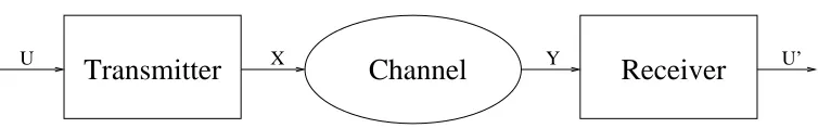
Figure 1.1: A canonical communication system.
1.1
Basics of channel coding
1.1.1
Channel capacity
A canonical model of a single transmitter, single receiver communication system, originally studied by Shannon, is shown in Figure 1.1. The objective is to send a sequence of symbols U = (4 U1, U2, ..., Uk) across the noisy channel. To do this, the
transmitter maps (or encodes) U to another sequence of bits X = (4 X1, X2, ..., Xn),
which it then transmits over the channel. The receiver sees a string of corrupted output symbols Y = (4 Y1, Y2, ..., Yn) where Y depends on X via a probability density
function (pdf) pY|X(y|x). The receiver then estimates (or decodes)U based on Y.
Definition 1.1 A channel is called memoryless if the channel output at any time instant depends only on the input at that time instant. Mathematically, this means that pY|X(y|x) = Qni=1pY|X(yi|xi). In this case, the channel is completely described
by its input and output alphabets, and the conditional pdf pY|X(y|x) for one time
instant.
If each Xi is chosen independently and identically distributed (i.i.d.) according to a
pdf pX(x), then the Yi’s are also i.i.d., with the pdf pY(y) given by
pY(y) =
Z
X
Definition 1.2 The mutual information between the random variables X and Y, denoted by I(X;Y) is defined as
I(X;Y) = Z
X,Y
p(x)p(y|x) log2
p(y|x)
p(y)
dx dy (1.2)
The mutual information between X and Y is a quantitative measure of what the knowledge of Y can tell us about X (and vice versa).
Definition 1.3 The capacityof a memoryless channel specified by pY|X(y|x) is
C = sup
pX(x)
I(X;Y) (1.3)
Intuitively, C is the maximum of amount of information that can be learnt about X
from Y and hence is a measure of the maximum rate R at which information can be reliably transmitted across the channel. Shannon rigorously showed this was the case [10, 71], i.e., error free transmission was possible at rates R < C and impossible at rates R > C, where R and C are both measured in bits per channel use.
1.1.2
Channel models
In this thesis, we focus on binary input symmetric channels (BISCs) viz., channels with the input X chosen from a binary input alphabet and the output symmetric in the input. We interchangeably use the sets {0,1} and {+1,−1} for the input alphabet with 0 mapping to +1 and 1 to −1. The symmetry condition implies that
pY|X(y|+ 1) = pY|X(−y| −1). We now present three of the most important BISCs,
which arise in many communication systems.
1−p and is 0 with probability p. p is called the probability of erasure. This channel is arguably the simplest nontrivial channel model, and has capacity 1−p.
Example 1.2 (The binary symmetric channel (BSC)) This is a binary-input, binary-output channel with parameter p. To view it as a BISC, it is convenient to let the input and output alphabets be {+1,−1}. Then the output is equal to the input with probability 1−p, and is the negative of the input with probability p. p is called the crossover probability of the channel. The capacity of this channel is given by 1−H(p), where H(p) is the entropy function −plog2p−(1−p) log2(1−p). Example 1.3 (The binary input additive white Gaussian noise channel
(BI-AWGNC))The binary input additive white Gaussian noise channel has inputsX re-stricted to inputs +1 and -1. The outputY is a random variable given byY =X+N, whereN is a Gaussian random variable with mean zero and varianceσ2. The capacity
of the AWGNC is given by
C= 1− √ 1
2πσ2
Z
R
H
1 1 +e2x/σ2
e(x2−σ1)22 dx (1.4)
where H(·) is again the entropy function. It is customary to express the capacity of a BIAWGNC in terms of its signal-to-noise ratio (SNR) defined as
Es
N0
= 10 log10
1 2σ2
dB
Eb
N0
= 10 log10
1 2Cσ2
dB (1.5)
Here Es/N0 denotes the SNR per transmitted bit and Eb/N0 denotes the SNR per
1.1.3
Channel codes
A channel code is defined as a mapping from a set of messagesM={1,2, ..., M} to a set of codewords, which are vectors of length n over some alphabet A. n is called the blocklength of the code and log2M its dimension.
The most common channel codes are binary codes in which the alphabet A =
{0,1}and M = 2k for some k. In such a case, we refer to the code as a (n, k) code.
The rate R of the code is defined as k/n. A binary code can also be thought of as a mapping from{0,1}kto{0,1}n. In other words, a channel code maps ak-bit message
to an n-bit codeword. Most practical channel codes have n > k, which means that
n−k redundant bits are added to the message. It is this redundancy that helps in error correction.
Often, we need to impose additional structure on the codes to make them easier to design, analyze and implement. Most practical codes in use today arelinearcodes.
Definition 1.4 An (n, k) linear code over the binary fieldGF(2) is a k-dimensional vector subspace of GF(2)n.
Linear codes have several nice properties, for example, they look exactly the same around any codeword. That is, if C is a linear code and c ∈ C is a codeword, then the set C −c is identical to C. Also, in order to describe a linear code, we don’t have to list all its elements, but merely a basis. Such a description is called a generator matrix representation.
Definition 1.5 A generator matrix for an (n, k) linear code C is a k×n matrix G
whose rows form a basis for C. As u varies over the space GF(2)k, uG varies over
the set of codewords. Thus, the matrix G provides a simple encoding mechanism for the code.
Definition 1.6 A parity-check matrix (PCM) for an (n, k) linear code C is an (n− k)×n matrix H whose rows form a basis for the space of vectors orthogonal to C. That is, H is a full rank matrix s.t. Hc=0 ⇐⇒ c∈ C.
The parity check matrix representation can be represented graphically using a bipar-tite graph called a Tanner graph. Each row i of the PCM corresponds to a check node, and each column j to a variable node. There is an edge between check node i
and variable node j if and only if Hij = 1.
Definition 1.7 TheHamming distancebetween two vectors is the number of compo-nents in which they differ. Theminimum distance of a code is the smallest Hamming distance between two distinct codewords. For a linear code, this is the same as the least weight of any nonzero codeword.
1.1.4
Capacity achieving codes
Even for moderately largek, there are a very large number of channel codes. Finding
capacity achieving codes, informally defined as codes with low probability of error and rates close to channel capacity, from this large set of codes seems like a computation-ally impossible task. However, Shannon showed that the ensemble of random codes
can achieve capacity as k → ∞ [10]. A random code is one in which each message is mapped to a codeword picked randomly according to a uniform distribution on
{0,1}n. It can also be shown that the ensemble of random linear codes can achieve
capacity on any BISC. In a random linear code, each of the n codeword bits is gen-erated by taking a random linear combination of the k data bits. In other words, each element of the generator matrixG(or the parity check matrixH) is chosen i.i.d. according to the distribution Pr(0) = Pr(1) = 1/2.
codes and random linear codes can achieve capacity under maximum-likelihood (ML) decoding, an algorithm whose complexity grows exponentially ink. Given the received sequence Y, the ML-decoder searches the entire codeword space (consisting of 2k
words) and outputs
ˆ
x= arg max
x∈C
pY|X(y|x). (1.6)
Clearly, the ML-decoder is optimal in the sense that it minimizes theword error rate
(WER), which is the probability ˆxis not the same as the transmitted codeword. ML-decoders are hard to implement for most codes since ML-decoding typically involves computing pY|X(y|x) for all 2k codewords. It must be noted here that there are
classes of codes which can be ML-decoded in polynomial time. An example would be convolutional codes [17], whose ML-decoding algorithm is the Viterbi algorithm [81] whose complexity is linear in the length of the code. However, practical convolutional codes are not capacity achieving.
1.2
Low density parity check codes
The high complexity associated with ML-decoding of random linear codes creates the need for capacity-achieving codes with efficient decoding algorithms. Such codes could not be found despite the invention of a large number of code families [53, 82] with efficient decoding algorithms. The situation changed in 1993 with invention of turbo codes [5], which led to the design of capacity-achievinglow density parity check
(LDPC) codes. We will now describe the structure of these codes and their decoding algorithms.
RANDOM PERMUTATION OF EDGES Left degree = 3
Right degree = 6
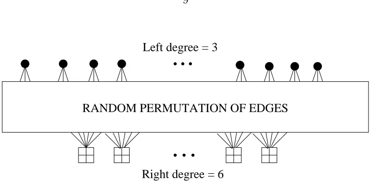
Figure 1.2: Tanner graph of (3,6)-regular LDPC code.
aroundn/2 or O(n) ones per row. This means that each variable node in the Tanner graph of an LDPC code is connected to O(1) check nodes, and each check node is connected to O(1) variable nodes.
The simplest kind of LDPC codes are regular LDPC codes. In a (dv, dc)-regular
LDPC code, each variable node is connected to exactlydv check nodes and each check
node is connected to exactlydcvariable nodes. The connections between the variable
nodes and check nodes are generally chosen at random. For largen, the rate of such a code is 1−dv/dc. Figure 1.2 shows the Tanner graph of a (3,6)-regular LDPC code.
1.2.1
Degree distributions
A more general class of LDPC codes areirregularLDPC codes. In an irregular LDPC code, different nodes may have different connectivities. For example, half the variable nodes may be connected to two check nodes each, a quarter to three check nodes each, and the remaining quarter to eight check nodes. Thevariable node degree distribution
of such a code is specified by the polynomial ν(x) = 0.5x2 + 0.25x3 + 0.25x8. The
ν(x) =xdv and µ(x) =xdc.
We can also define the edge degree distributions λ(x) and ρ(x).
λ(x) = ν
0
(x)
ν0
(1)
ρ(x) = µ
0
(x)
µ0
(1) (1.7)
For the (3,6)-LDPC code, λ(x) = x2 and ρ(x) = x5. λ(x) = x2 means that an edge
has two neighboring edges at the variable node side, i.e., two edges connected to the same variable node. Similarly, ρ(x) = x5 means that five neighboring edges at the
check node side. For an irregular LDPC code, the polynomials λ(x) andρ(x) specify probability distributions on edge connectivities. Edge distribution polynomials are more useful in analyzing code performance than node distribution polynomials. This is because of the nature of the algorithm used to decode LDPC codes.
1.2.2
Iterative decoding
The iterative decoding algorithm used to decode LDPC codes, called thesum-product algorithm, is a completely distributed algorithm with each node acting as an indepen-dent entity communicating with other nodes through the edges. The message sent by a variable node to a check node is its estimate of its own value. Typically the messages are sent inlog-likelihood ratio(LLR) form. The LLR of any bit is defined as log(Pr(bit = 0)/Pr(bit = 1)). The message sent by a check node to a variable node is the check node’s estimate of the variable node’s value.
At a variable node of degree j, if l1, l2, . . . , lj−1 denote the incoming LLRs along
j−1 edges, and l0 the LLR corresponding to the channel evidence, then the outgoing
LLR lout along the jth edge is merely the maximum a posteriori (MAP) estimate of
given by
lout =l0+
j−1
X
i=1
li. (1.8)
At a check node, the situation is similar, though the update rule is more complicated. If l1, l2, . . . , lk−1 denote the incoming LLR’s at a check node of degree k, then the
outgoing LLR lk along thekth edge corresponds to the pdf of the binary sum ofj−1
independent random variables, and works out to be
tanh(lout/2) =
k−1
Y
i=1
tanh(li/2). (1.9)
(For a derivation of eqs. (1.8) and (1.9), see [66, Section 3.2].)
1.2.3
Capacity achieving distributions
Since a message is passed along each edge in every iteration of the sum-product algorithm, the complexity of decoding (per iteration) is proportional to the number of edges in the Tanner graph. Since the graph is sparse, the number of edges and thus the decoding complexity (per iteration) grow linearly in n. This allows for the decoding of codes with very high blocklengths. Therefore, all that remains to be done is the design of LDPC codes which can achieve capacity under iterative decoding.
It can be shown using density evolution analysis [45, 66] that such design is indeed feasible. The proof consists of three main steps. Firstly, it can be shown that the performance of an ensemble of LDPC codes depends only on its degree distribution in the limit of infinite blocklength. This is not hard to understand because the connections between the variable nodes and check nodes are chosen at random. The second step is show that an ensemble has athresholdchannel parameter. For example, codes designed using the (3,6)-regular distribution have a threshold of p= 0.429 on the BEC. This means that the average bit error rateof the code ensemble approaches zero asn → ∞when the codes are used on a BEC with probability of erasure less than 0.429. For comparison, a capacity-achieving random linear code under ML-decoding has a threshold of p= 0.5. This means that the (3,6)-code ensemble is not capacity achieving.
within 0.0045 dB of channel capacity on the BIAWGNC [8]. While these codes are not strictly capacity-achieving, their thresholds are close enough to channel capacity for all practical purposes.
While density evolution allows us to design asymptotically good degree distribu-tions, it does not guarantee that these codes work well at finite block lengths. How-ever, extensive simulation studies have shown that LDPC codes have very good perfor-mance in the intermediate blocklength (n ≈1000) to long blocklength (n ≈100000) range [9]. They perform rather poorly in the short block length (n < 1000) range. However, since iterative decoding is extremely fast, it is possible to use long codes in practice. For example, Flarion Technologies designed an LDPC code with n = 8192 and rate 1/2 that has a WER of 10−10 at under 1.5 dB from capacity on the
BI-AWGNC. The hardware implementation of their decoder can support data rates up to 10 Gbps [18].
1.3
Thesis outline
The results stated in Section 1.2.3 might lead us to the conclusion that the problem of transmitting data reliably and efficiently over noisy channels has been solved. Such a conclusion would not be untrue for the communication system shown in Figure 1.1 where a single transmitter transmits data to a single receiver over a channel whose statistics are known a priori to both the transmitter and the receiver. However, not all communications systems can be characterized by such a simple model.
Transmitter
Transmitter Receiver
Receiver Receiver
Receiver + Transmitter
Transmitter +
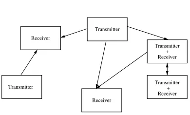
Figure 1.3: A general communication system.
time, and the channel statistics may not be known to the nodes. Moreover, if the network is wireless, transmissions from multiple senders can interfere at a receiver.
Since many contemporary communication systems are in fact networks, we would like to design efficient error correction codes for general networks. Unfortunately, this is very hard for two reasons. Firstly, the capacity region of a general network is not known [10, Chapter 14]. Secondly, even in the special cases where the capacity region is known, it is not clear that efficient capacity achieving codes exist. In this thesis, we take a few steps towards the design of efficient network codes. Our approach is twofold: in cases where the capacity region of the network is known, we study the performance of LDPC-like codes under iterative decoding. In cases where the capacity region is unknown, we try to compute the capacity region.
The rest of the thesis is organized as follows. In Chapter 2, we study the perfor-mance of rateless codeson the BSC and the BIAWGNC. These codes are designed to be used on time varying channels where the channel statistics are not known a priori to the transmitter and the receiver. An ideal rateless code should work well on any channel, no matter how good or bad the channel is. We show that this is the case for a class of codes called raptor codes.
senders interfere with each other at the receiver. We describe how the sum-product algorithm can be adapted to handle such interference, and how LDPC codes can be designed for a MAC.
In Section 1.2.3, we mentioned that LDPC codes perform poorly at short block-lengths. In Chapter 4, we design iterative decoding algorithms for a class of non-sparse codes calledEuclidean geometry (EG) codes. We show that some short EG codes ex-hibit excellent performance under these algorithms. More generally, we show that it is possible to decode non-LDPC codes using iterative decoding.
In Chapter 5, we study a class of wireless relay networks for which the capacity region was previously unknown. In these networks, a single source wants to transmit information to a single receiver. All the other nodes act as relays, which aid in the communication between the transmitter and the receiver. We derive the capacity of such a network under certain conditions.
In Chapter 6, we study fading channels, which are very common in wireless net-works. We study the capacity-achieving distributions of certainblock fadingchannels, and show that the capacity achieving distributions of all block fading channels have some common theoretical properties.
Chapter 2
Rateless codes on noisy
channels
In this chapter, we consider iterative decoding for channels when the transmitter and receiver have no prior knowledge of the channel statistics. We give a brief description of rateless codes and go on to study the performance of two classes of rateless codes (LT and raptor codes) on noisy channels such as the BSC and the AWGNC. We find that raptor codes outperform LT codes, and have good performance on a wide variety of channels.
2.1
Introduction
decoding failure when used over a bad channel (highp). Conversely, a code designed for a bad channel would result in unnecessary packet transmissions when used over a good channel.
This problem can be solved using rateless codes. Instead of encoding thek infor-mation bits to a pre-determined number of bits using a block code, the transmitter encodes them into a potentially infinite stream of bits and then starts transmitting them. Once the receiver gets a sufficient number of symbols from the output stream, it decodes the originalk bits. The number of symbols required for successful decoding depends on the quality of the channel. If decoding fails, the receiver can pick up a few more output symbols and attempt decoding again. This process can be repeated until successful decoding. The receiver can then tell the transmitter over a feedback channel to stop any further transmission.
The use of such anincremental redundancyscheme is not new to coding theorists. In 1974, Mandelbaum [50] proposed puncturing a low rate block code to build such a system. First the information bits are encoded using a low rate block code. The resulting codeword is then punctured suitably and transmitted over the channel. At the receiver the punctured bits are treated as erasures. If the receiver fails to decode using just the received bits, then some of the punctured bits are transmitted. This process is repeated till every bit of the low rate codeword has been transmitted. If the decoder still fails, the transmitter begins to retransmit bits till successful decoding. It is easy to see such a system is indeed a rateless code, since the encoder ends up transmitting a different number of bits depending on the quality of the channel. Moreover, if the block code is a random (or random linear) block code, then the rateless code approaches the Shannon limit on every binary input symmetric channel (BISC) as the rate of the block code approaches zero. Thus such a scheme is optimal in the information theoretic sense.
origi-nally used Reed-Solomon codes for this purpose and other authors have investigated the use of punctured low rate convolutional [27] and turbo [39] codes. In addition to many code-dependent problems, all these schemes share a few common problems. Firstly, the performance of the rateless code is highly sensitive to the performance of the low rate block code, i.e., a slightly sub-optimal block code can result in a highly sub-optimal rateless code. Secondly, the rateless code has very high decoding complexity, even on a good channel. This is because on any channel, the decoder is decoding the same low rate code, but with varying channel information. The com-plexity of such a decoding scheme grows at least as O(k/R) where R is the rate of the low rate code.
In a recent landmark paper, Luby [43] circumvented these problems by designing rateless codes which are not obtained by puncturing standard block codes. These codes, known as Luby Transform(LT) codes, are low density generator matrix codes which are decoded using the same message passing decoding algorithm (belief prop-agation) that is used to decode LDPC codes. Also, just like LDPC codes, LT codes achieve capacity on every BEC. Unfortunately, LT codes also share the error floor
problem endemic to capacity achieving LDPC codes. Shokrollahi [73] showed that this problem can be solved using raptor codes, which are LT codes combined with outer LDPC codes. These codes have no noticeable error floors on the BEC. However, their rate is slightly bounded away from capacity.
2.2
Luby transform codes
The operation of an LT encoder is very easy to describe. From k given information bits, it generates an infinite stream of encoded bits, with each such encoded bit gen-erated as follows:
1. Pick a degree d at random according to a distribution µ(d). 2. Choose uniformly at random d distinct input bits.
3. The encoded bit’s value is the XOR-sum of these d bit values.
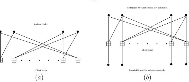
The encoded bit is then transmitted over a noisy channel, and the decoder receives a corrupted version of this bit. Here we make the non-trivial assumption that the en-coder and deen-coder are completely synchronized and share a common random number generator, i.e., the decoder knows which d bits are used to generate any given en-coded bit, but not their values. On the Internet, this sort of synchronization is easily achieved because every packet has an uncorrupted packet number. More complicated schemes are required on other channels; here we shall just assume some such scheme exists and works perfectly in the system we’re studying. In other words, the decoder can reconstruct the LT code’s Tanner graph without error.
Check nodes Variable Nodes
!! ""#"#
$$%$% &'&' (( )) ** ++
Information bit variable nodes (not transmitted)
Check nodes
Encoded bit variable nodes (transmitted)
(a) (b)
Figure 2.1: Tanner graph of (a) LDPC code (b) LT code.
2.2.1
The robust soliton distribution
Clearly, for large block lengths, the performance of such a system depends mostly on the degree distribution µ. Luby uses the Robust Soliton (RS) distribution, which in turn is based on the ideal soliton distribution, defined as follows:
ρ(1) = 1/k
ρ(i) = 1/i(i−1) ∀i∈ {2,3, ..., k} (2.1)
While the ideal soliton distribution is optimal in some ways (cf. [43]), it performs rather poorly in practice. However, it can modified slightly to yield the robust soliton distribution RS(k, c, δ). Let R =4 c·ln(k/δ)√k for some suitable constant c > 0. Define
τ(i) =
R/ik for i= 1, . . . , k/R−1
Rln(R/δ)/k for i=k/R
0 for i=k/R+ 1, . . . , k
(2.2)
Now addτ(.) to the ideal soliton distribution ρ(.) and normalize to obtain the robust soliton distribution:
distri-bution.
Luby’s analysis and simulation studies show that this distribution performs very well on the erasure channel. The only disadvantage is the decoding complexity grows asO(klnk), but it turns out that such a growth in complexity is in fact necessary to achieve capacity [73]. However, slightly sub-optimal codes called raptor codes, can be designed with decoding complexity O(k) [73]. On the BEC, theoretical analysis of the performance of LT codes and raptor codes is feasible, and both codes have been shown to have excellent performance. In fact, raptor codes are currently being used by Digital Fountain, a Silicon Valley based company, to provide fast and reliable transfer of large files over the Internet.
On other channels such as the BSC and the AWGNC, there have been no studies in the literature on the use of LT and raptor codes, despite the existence of many potential applications, e.g., transfer of large files over a wireless link, multicast over a wireless channel. We hope to fill this void by presenting some simulation results and some theoretical analysis (density evolution). In this chapter, we focus on the BSC and the AWGNC, but we believe that our results can be extended to time varying and fading channels.
2.3
LT codes on noisy channels
When the receiver tries decoding after picking up a finite number n of symbols from the infinite stream sent out by the transmitter, it is in effect trying to decode an (n, k) code, with a non-zero rate R = k/n. As R decreases, the decoding complexity goes up and the probability of decoding error goes down. In this chapter, we have studied the variation of bit error rate (BER) and word error rate (WER) with the rate of the code on a given channel.
2 2.1 2.2 2.3 2.4 2.5 2.6 2.7 2.8 2.9 3 10−3
10−2 10−1 100
R−1
WER / BER
LT codes on BSC with p=0.11
k=1000 WER k=1000 BER k=10000 WER k=10000 BER
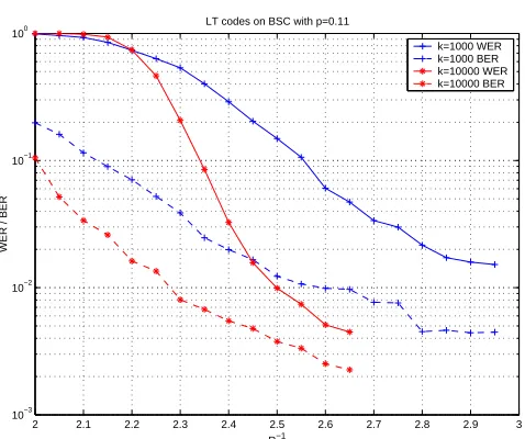
Figure 2.2: The performance of LT codes generated using the RS(k,0.01,0.5) distri-bution on a BSC with p= 0.11.
probability. We mention that the results are similar in nature on other BSCs and other AWGNCs as well. In this figure, we plot R−1 on the x-axis and BER/WER
on the y-axis. The receiver buffers up kR−1 bits before it starts decoding the LT
code using belief propagation. On a BSC with 11% bit flip probability, the Shannon limit is R−1 = 2, i.e., a little over 2k bits should suffice for reliable decoding in the
large k limit. We see from the figure that an LT code with k = 10000 drawn using the RS(10000,0.1,0.5) distribution can achieve a WER of 10−2 at R−1 = 2.5 (or n =
25000). While this may suffice for certain applications, neither a 25% overhead nor a WER of 10−2is particularly impressive. Moreover, the WER and BER curves bottom
out into an error floor, and achieving very small WERs without huge overheads in nearly impossible. Going to higher block lengths is also not practical because of the
O(klnk) complexity.
2.3.1
Error floors
BEC1[73] also exhibit similar behaviour. The main advantage of these distributions
is that the average number of edges per node remains constant with increasing k, which means the decoding complexity grows only as O(k). On the minus side, there will be a small fraction of information bit nodes that are not connected to any check node. This means that even as k goes to infinity, the bit error rate does not go to zero and consequently, the word error rate is always one.
In this chapter, we discuss the performance of one particular distribution from [73]:
µ(x) = 0.007969x+ 0.493570x2+ 0.166220x3
+0.072646x4+ 0.082558x5+ 0.056058x8+ 0.037229x9
+0.055590x19+ 0.025023x65+ 0.0003135x66 (2.4)
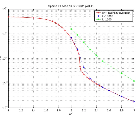
Shown in Figure 2.3 is the performance of codes generated using the distribution in equation (2.4) at lengths 1000, 10000 and infinity. The performance at length infinity is computed using density evolution [66]. Again, we observe fairly bad error floors, even in the infinite blocklength limit.
We must mention that these error floors are not just due to the presence of in-formation bit variable nodes not connected to any check nodes. For example, when
R−1 = 3.00, only a very small fraction of variable nodes (2.25×10⁻⁸) are unconnected,
while density evolution predicts a much larger bit error rate (1.75×10⁻⁴). This can
be attributed in part to the fact that there are variable nodes which are connected to a relatively small number of output nodes and hence are always unreliable.
1Note that these distributions were not designed to be used in LT codes, but in raptor codes.
1 1.2 1.4 1.6 1.8 2 2.2 2.4 2.6 2.8 3 10−4
10−3
10−2 10−1 100
R−1
BER
Sparse LT code on BSC with p=0.11
k=∞ (Density evolution) k=10000 k=1000
Figure 2.3: Performance of LT codes generated using right distribution given in equa-tion (2.4) on BSC with p= 0.11.
2.4
Raptor codes
The error floors exhibited by LT codes suggest the use of an outer code. Indeed this is what Shokrollahi does in the case of the BEC [73, 74] where he introduces2 the
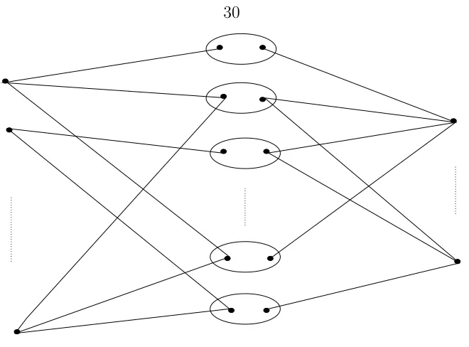
idea of raptor codes, which are LT codes combined with outer codes. Typically these outer codes are high rate LDPC codes. In this chapter, we use the distribution in equation (2.4) for the inner LT code. For the outer LDPC code, we follow Shokrollahi [73] and use a left regular distribution (node degree 4 for all nodes) and right Poisson (check nodes chosen randomly with a uniform distribution).
The encoder for such a raptor code works as follows: the k input bits are first encoded into k0 bits to form a codeword of the outer LDPC code. These k0 bits are then encoded into an infinite stream of bits using the rateless LT code. The decoder picks up a sufficient number (n) of output symbols, constructs a Tanner graph that incorporates both the outer LDPC code and the inner LT code, and decodes using belief propagation on this Tanner graph.
2We must mention here that Maymounkov [52] independently proposed the idea of using an outer
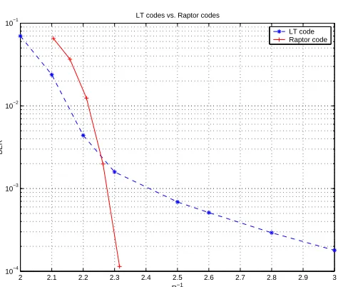
2 2.1 2.2 2.3 2.4 2.5 2.6 2.7 2.8 2.9 3 10−4
10−3 10−2 10−1
R−1
BER
LT codes vs. Raptor codes
LT code Raptor code
Figure 2.4: Comparing LT codes with raptor codes on a BSC with p=0.11. The LT code has k = 10000 and is generated using the distribution in equation (2.4). The raptor code has k = 9500 and has two components: an outer rate-0.95 LDPC code and an inner rateless LT code generated using the distribution in equation (2.4).
Simulation studies, such as the one shown in Figure 2.4, clearly indicate the supe-riority of raptor codes. Figure 2.4 shows a comparison between LT codes and raptor codes on a BSC with bit flip probability 0.11. The LT code has k = 10000 and is generated using the distribution in equation (2.4). The raptor code hask= 9500 and uses an outer LDPC code of rate 0.95 to get k0 = 10000 encoded bits. These bits are then encoded using an inner LT code, again generated using the distribution in equation (2.4). Figure 2.4 clearly shows the advantage of using the outer high rate code.
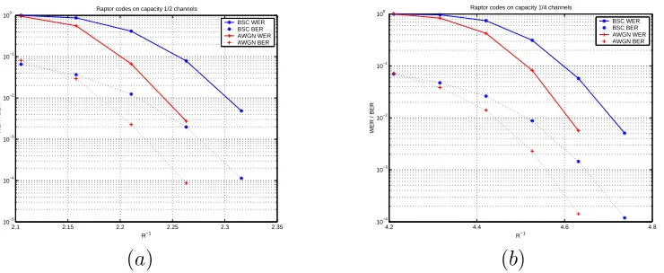
Raptor codes not only beat LT codes comprehensively, but also have near-optimal performance on a wide variety of channels as shown in Figure 2.5, which shows the performance of the aforementioned raptor code on four different channels. On each of these channels, the raptor code has a waterfall region close to the Shannon capacity, with no noticeable error floors. Of course, this does not rule out error floors at lower WERs.
2.1 2.15 2.2 2.25 2.3 2.35 10−5 10−4 10−3 10−2 10−1
100 Raptor codes on capacity 1/2 channels
R−1
WER / BER
BSC WER BSC BER AWGN WER AWGN BER
4.2 4.4 4.6 4.8
10−4
10−3
10−2
10−1
100 Raptor codes on capacity 1/4 channels
R−1
WER / BER
BSC WER BSC BER AWGN WER AWGN BER
(a) (b)
Figure 2.5: Performance of raptor code with k=9500 and k’=10000 on different chan-nels: (a) BSC with p = 0.11 and AWGNC with Es/N0 = −2.83dB. Both channels
have capacity 0.5. (b) on BSC withp= 0.2145 and AWGNC withEs/N0 =−6.81dB.
Both channels have capacity 0.25
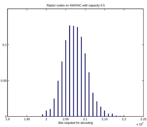
number of bits required for successful decoding. We must note here this indicator not only depends on the code, but also on the number of decoding attempts made by the receiver. For example, the decoder could attempt decoding each time it receives a new noisy bit. While such a decoder would be optimal in terms of number of bits required for successful decoding, it would have prohibitively high decoding complexity. A more practical decoder would wait for more bits to come in before decoding. Such a decoder would have a vastly lower complexity at the expense of slightly larger number of bits received. Note that there is no need for such a tradeoff in the case of the BEC. This is because the decoder fails when the Tanner graph is reduced to a stopping set[13]. After new bits are received, further decoding can be done on the stopping set instead of the original Tanner graph. Such a scheme is not appplicable to noisy channels where the decoder must start over every time new bits are received.
1.9 1.95 2 2.05 2.1 2.15 2.2 2.25 x 10⁴ 0
0.05 0.1
Bits requited for decoding Raptor codes on AWGNC with capacity 0.5
Figure 2.6: Histogram of number of bits required for successful decoding of raptor code with k = 9500 on an AWGNC with Es/N0 = −2.83dB. The capacity of this
channel is 0.5. The receiver first attempts decoding after receiving 19000 noisy bits (Shannon limit). Whenever decoding fails, the receiver waits for another 100 bits before attempting to decode again.
2.5
Conclusion
We have conducted simulation studies and density evolution analysis of rateless codes on channels such as the BSC and the AWGNC. We found that raptor codes have excellent performance on such channels, while the performance of LT codes is not as good. These results suggest that raptor codes are ideal for use in data transfer protocols on noisy channels. A similar observation has already been made on the BEC [73] and consequently, commercial applications that use raptor codes on the Internet are already in the market.
Chapter 3
Graph-based codes for
synchronous multiple access channels
In this chapter, we discuss a general algorithm for using LDPC-like codes on a syn-chronous multiple access channel (MAC). We then introduce a code design procedure known as graph-splitting, and show that codes designed using this technique achieve capacity on the binary adder channel (BAC) without using timesharing. Finally, we present simulation results for the noisy binary adder channel, qualitatively ana-lyze these results and argue that LDPC-like codes perform well on multiple access channels.
3.1
Introduction to multiple access channels
A multiple access channel (MAC) [10, Section 14.3] is defined as a channel in which two or more senders send information to the same receiver. Examples include a satellite receiver with many independent ground stations or a cellular base station receiving inputs from many cell phones. In these channels, the senders must not only contend with the receiver noise, but also interference from each other. In mathe-matical terms, a discrete memoryless MAC is defined as a channel that takes in n
inputs x1 ∈ X1, x2 ∈ X2, . . . , xn ∈ Xn and produces an output y ∈ Y according to a
probability transition matrix p(y|x1, x2, . . . , xn).
satisfying
R1 < I(X1;Y|X2),
R2 < I(X2;Y|X1),
R1+R2 < I(X1, X2;Y) (3.1)
for some product distributionp1(x1)p2(x2) on X1× X2. A detailed proof of this result
is found in [10, Section 14.3]. The key point to note here is that the input distribution should be a product distribution. This reflects the fact that the inputs X1 and X2
come from different users.
The MACs we consider in this chapter are synchronous, i.e., all users share a common clock. In a synchronous MAC, we can assume that the codeword length and codeword boundaries are the same for every user. We must mention the capacity region of an asynchronous MAC is the same as that of the corresponding synchronous MAC [11]; however, the coding scheme that achieves capacity is much simpler in the synchronous case.
3.2
Decoding LDPC codes on a MAC
In this section, we discuss a general algorithm for using low density parity check (LDPC) codes on a binary input two-user MAC. Assume that User 1 and User 2 encode their respective data independently using two distinct LDPC codes with same blocklength n and rates R1 and R2. At the channel output, we get a sequence of
symbols which is a probabilistic function of the two transmitted codewords. Based on the received channel symbol, we can compute channel information by using Bayes’ rule.
pch(x1, x2|y) =
p1(x1)p2(x2) p(y|x1, x2)
Check Nodes of Graph 1
Check Nodes of Graph 2 Variable Nodes
Figure 3.1: LDPC codes on a MAC: Each user encodes his data independently using an LDPC code, but the channel gives an output dependent on the bits from both users.
where x1, x2 ∈ {0,1} and y ∈ Y. Note that we have a joint distribution on the
possible channel inputs.
The belief propagation decoding algorithm proceeds as follows. At a check node (of either Graph 1 or Graph 2), the update rule is the same as in a single user LDPC code. The incoming bits to any check node should sum to zero, therefore the outgoing message along any edge is the convolution of the messages along all other incoming edges. Since the pmfs get convolved, their Fourier transforms get multiplied and therefore the outgoing message along any edge i is given by
Piout(x) = Y
j6=i
Pjin(x) (3.3)
At the variable nodes, each incoming message along the edges of Graph 1 is an independent estimate of the x1. Similarly, each incoming message along the edges
of Graph 2 is an independent estimate of x2. Moreover, if the two graphs are also
designed randomly, then with high probability, the messages coming in from both the graphs are also independent of each other. In addition to these messages, we also have the joint channel information. Therefore, by the usual belief propagation rule, we get the outgoing joint message along an edge i of Graph 1 to be
piout(x1, x2) ∝ pch(x1, x2)
Y
j16=i
pj1(x1)
Y
j2
pj2(x2) (3.4)
Thus, the joint message passed along an edge of Graph 1 depends on the channel information, all the incoming messages along the edges of Graph 2 connected to the corresponding variable node, and the incoming messages along all the edges of Graph 1 (except the edge along which the outgoing message is passed) connected to the same variable node. However, we do not want to pass this joint distribution along Graph 1 since we just need to pass a message about x1, so we marginalize the joint
distribution to get
piout(x1)∝
Y
j16=i
pj1(x1)
1
X
x2=0
pch(x1, x2)
Y
j2
pj2(x2)
!
(3.5)
Now we define the updated channel informationp0ch as follows:
p01ch(x1)∝ 1
X
x2=0
pch(x1, x2)
Y
j2
pj2(x2)
!
(3.6)
Note thatp0
ch does not depend on the edgeialong which the message is to be passed.
After computing the updated channel information, we pass messages as in a single-user LDPC code. The message along edgei is
piout(x1)∝p
0
1ch(x1) Y
j16=i
pj1in(x1) (3.7)
Similar update rules apply to Graph 2; using the incoming messages from Graph 1 and the joint channel information, we compute the updated channel information for Decoder 2.
p02ch(x2)∝ 1
X
x1=0
pch(x1, x2)
Y
j1
pj1(x1)
!
(3.8)
Then we pass messages on Graph 2 similar to a usual single-user LDPC code, i.e., in a manner similar to that in equation 3.7.
piout(x2)∝p
0
2ch(x2) Y
j26=i
pj2in(x2) (3.9)
We repeat the above iteration steps till a criterion for stopping is met. For example, the algorithm can be stopped when all the parity checks are satisfied or after a fixed number of iterations.
Thus the decoder for the MAC is the same as two single-user LDPC decoders with each decoder updating the effective channel information for the other code at each iteration. The MAC is very similar to the turbo decoder used to decode concatenated codes; just like the MAC decoder, a turbo decoder is comprised of two or more simple component decoders operating in tandem [5].
3.3
The binary adder channel
addition is over the real field. There is no ambiguity in (x1, x2) if y = 0 or if y = 2.
However y = 1 can result from either (x1, x2) = (0,1) or (x1, x2) = (1,0). Thus the
inputs are determined for two of the possible output values, but are ambiguous for the third. This is why the BAC is sometimes referred to as the binary erasure multiple access channel.
The capacity of the BAC can be computed very easily from equations (3.1). It turns out the capacity of the BAC [10] is given by
R1 <1, R2 <1, R1+R2 <1.5 (3.10)
Therefore it is possible to achieve a joint rate of 1.5 bits per channel use. We now consider our algorithm on the BAC. Suppose User 1 encodes his data with an LDPC code of rate R1 and User 2 does the same with a code of rate R2. Let n be the
blocklength of both the codes. Since both bitstreams are independent, the weak law of large numbers tells us that with high probability, the channel input would have an equal number (i.e.,n/4) of the four possible bit pairs (0,0),(0,1),(1,0) and (1,1). Since (0,1) and (1,0) result in the same output Y = 1, at the channel output we would see n/4 0s,n/2 1s, andn/4 2s. To either decoder, this looks liken/4 0s,n/4 1s andn/2 erasures, i.e., like the output of a erasure channel with probability of erasure 1/2. However, the erasures input to both the decoders are dependent and decoding an erasure in one user’s codeword would automatically decode the corresponding erasure in the other user’s codeword.
erasure to that incoming non-erasure, (2) at a check node, if all except one incoming messages are non-erasures, then decode that erasure to be the sum over GF(2) of all the other incoming messages. If there are more than one incoming erasures, then the check node just passes back erasures.
Our algorithm for the BAC works exactly the same way, except that the two LDPC decoders interact. The algorithm proceeds as follows: Do one iteration on each graph, thereby correcting some erasures on the input to Graph 1 and some other erasures on the input to Graph 2. Now erasures corrected on one graph are corrected on the other also. This corresponds to the “update channel information” step of the algorithm for the general MAC. Repeat this procedure till there are no erasures left or till no further erasures can be corrected.
3.4
Design of LDPC codes for the BAC
All that remains to be done is to find good LPDC codes for both the users. For this purpose, we introduce a graph-splitting design. We start with a good erasure correcting code of rateR < 1/2 having a Tanner graphG. We first split the set of check nodes C into two disjoint sets C1 and C2 having c1 and c2 check nodes respectively.
We now split the graphG into two disjoint graphsG1 andG2 whereG1 is the set of all
edges connected to the check nodes in C1 and G2 is the set of all edges connected to
the check nodes in C2. Now let G1 be the Tanner graph of User 1’s LDPC code and
G2 be the Tanner graph of User 2’s LDPC code. The rates of the codes are given by
R1 = 1−c1/n, R2 = 1−c2/n (3.11)
+
+
+
x1 x2 x3 x4 x5 x6+
+
+
+
x1 x2 x3 x4 x5 x6+
+
+
+
x1 x2 x3 x4 x5 x6 w1 w2 w3 w4 w5 w6+
(a) (b) (c)
Figure 3.2: The graph-splitting technique: (a) Start with the Tanner graph of a single user LDPC code (b) Split the graph into two subgraphs containing disjoint sets of check nodes (c) The two subgraphs are now the the Tanner graphs for the two users.
Thus, splitting a rate-Rgraph gives a joint graph of rate 1 +R. Therefore, if we split a “good” rate-1/2 erasure code, we get a joint rate of 1.5, which is the capacity of the BAC. What remains to be shown, of course, is that this graph-splitting design works. This is done by density evolution [66] analysis of the joint decoder.
3.4.1
Density evolution on the BAC
Suppose the probability that an erasure is passed along an edge of a graph to a check node isx. The message passed out of a check node is also an erasure when at least one of the other messages is an erasure. This occurs with probability y = 1−ρ(1−x), where ρ is the right degree sequence polynomial of the graph and equals xa−1 in
0.7 0.8 0.9 1 10−4
10−3
Rate R1
BER
Variation of BER with R
1 for constant R1 + R2 = 1.4456
1.43 1.44 1.45 1.46 1.47 1.48 1.49 1.5 10−4
10−3 10−2
10−1
100
Total Rate R1 + R2
BER
Performance on the BAC of IRA codes designed by graph−splitting
(a) (b)
Figure 3.3: Performance of graph-split codes: (a) Variation of BER with R1 for
constant overall rate R (b) Variation of BER with total rate R at rates close to capacity.
G. Thus the density evolution goes as follows:
x−→1−ρ(1−x) at the check nodes. (3.13)
x−→0.5λ(x) at the variable nodes. (3.14)
x−→0.5λ(1−ρ(1−x)) in one iteration. (3.15)
codes achieve capacity on the BEC. Therefore, we can state the following result: Codes designed by graph-splitting achieve capacity on the binary adder channel.
We used irregular repeat accumulate (IRA) codes [33] to test our graph-splitting code design and decoding algorithm on the BAC. IRA codes are very similar to LDPC codes, and have the extra advantage that they can be encoded in linear time. We used codes of length 10000 and constant right-degree 5 IRA codes. The simulations confirm the fact that the final probability of error does not depend on the individual
R1 and R2, but only on the joint rate R1+R2, i.e., it depends only on the graph G
and not the way it is split into subgraphs (see Figure 3.3a). A graph showing the performance of the codes at joint rates close to capacity is also shown (see Figure 3.3b).
3.5
The noisy binary adder channel
We now consider the noisy binary adder channel (noisy BAC) whose outputyis given by
y=x1 +x2+n (3.16)
wherex1, x2 ∈ {−1,+1}are the inputs from the users andn is a zero-mean Gaussian
random variable with variance σ2. Thus, in addition to the interference between the
two users, noise is also present at the receiver. The variation of the capacity region of the noisy BAC with Eb/N0= 10 log10(1/(R1+R2)σ2) is shown in Figure 3.4.
We now study the performance of LDPC-like codes on this channel. Our first choice for the two users’ codes would be those designed by graph-splitting, since they work well on the BAC. However, it turns out that these codes do not work at all on the noisy BAC. More precisely, we can show that the bit error probability is bounded away from zero for any noise variance σ2 >0.
0 0.5 1 1.5 0
0.5 1 1.5
Capacity Region of the Noisy BAC
R1
R2
R=1.5, Eb/N0=α
R=1.0, Eb/N0=2.2
R=0.5, Eb/N0=0.51
-2 2 4 6 8
SNR 0.2
0.4 0.6 0.8 1 1.2 1.4 1.6 Rate
(a) (b)
Figure 3.4: Capacity region of the noisy BAC: (a) The capacity region of the noisy BAC for three values of Eb/N0 (b) Plot showing the maximum achievable rate for a
given Eb/N0 and the R1, R2 coordinates of an extremal point of the capacity region
at that Eb/N0.
from the graph-splitting design. By splitting any graph G, there would be a non-zero fractionf of nodes for which all of the connected edges are in one of the subgraphs, say
G2(see Figure 3.2). For these nodes, onlyx2 (viz., the node with the edges connected)
can be corrected because only it participates in the belief propagation process. Now even if we assume x2 is perfectly decoded to +1 or −1 (which certainly need not be
the case), the resulting effective single user channel for User 1 is y=x1+n. Among
the unprotected bits of User 1, there will be a non-zero fractionQ(σ−1) of errors. On
the whole there will at least be a non-zero fraction of errorsf Q(σ−1)>0 of errors in
User 1’s bit stream. Therefore graph-splitting in its present form does work for the noisy BAC. A simple extension of this argument will show that this is the case for any noisy MAC, i.e., a MAC in which the output is not a deterministic function of both the inputs.
The next choice would be independently designed single-user LDPC codes with parameters (λ1(x), ρ1(x)) and (λ2(x), ρ2(x)). Assuming the coefficients ofx0andx1in
λ1(x) andλ2(x) are zero (an essential condition for a good single-user LDPC code), we
2 3 4 5 6 7 8 9 10−7
10−6 10−5 10−4 10−3 10−2
Eb/N0
BER
Performance of IRA codes with n=10000, R1+R2=1 on the noisy BAC
R1=0.65,R2=0.35 R1=0.5,R2=0.5 Capacity=2.2dB
Figure 3.5: Performance of IRA Codes on the noisy BAC at R1+R2 = 1.
achieve capacity on the BAC, except in the extreme case when (R1, R2) = (1.0,0.5)
or (0.5,1.0). Therefore, we would expect something similar in the case of the noisy BAC as well.
We again used IRA codes to test this hypothesis. SNR vs. BER performance curves for total rateR = 1 are shown in Figure 3.5. As we can see, the independently designed codes perform well when the ratesR1 andR2are close to the extremal points
of the capacity region and poorly when the rates R1 and R2 are equal.
The above result can be explained qualitatively as follows. An extremal point of any MAC is the rate pair (I(X1;Y), I(X2;Y|X1)) (or the similar pair with X1 and
X2 interchanged). This shows that X1 can be decoded independently first, because
the capacity of the single-user channel that User 1 sees is I(X1;Y). Based on the
decoded X1, we can decode X2 because the capacity of the single-user channel that
User 2 sees now is I(X2;Y|X1), since X1 has already been decoded. Therefore the
other. This method of decoding is known as successive cancellation or onion peeling [67]. Only the extremal points of the rate region of the MAC can be decoded by successive cancellation.
In the case of the independently designed LDPC codes on the noisy BAC, the extremal points can be decoded by using two single-user LDPC decoders. Since single-user LDPC codes are known (though not provably) to do extremely well, we expect good performance for these codes at the extremal point rates of the MAC as well. Note that we did not actually use a successive cancellation decoder in our simulations. Instead, we used the joint decoder described in Section 3.2. Since the joint decoder performs at least as well as the successive cancellation decoder, the performance for the extremal point is good. There is no reason however to believe that the same will be true for the non-extremal points. This explains the performance curves in Figure 3.5.
By timesharing the extremal rate pairs, we can achieve any rate pair in the ca-pacity region. This shows that LDPC-like codes exhibit good performance for any rate-pair on the noisy BAC. Also note that all the above arguments apply to any MAC and not just the noisy BAC.
3.6
Conclusion
Chapter 4
Iterative decoding of
multi-step majority logic decodable codes
In this chapter, we investigate the performance of iterative decoding algorithms for multi-step majority logic decodable (MSMLD) codes of intermediate length. We introduce a new bit-flipping algorithm that is able to decode these codes nearly as well as a maximum likelihood decoder on the binary symmetric channel. MSMLD codes decoded using bit-flipping algorithms can out-perform comparable BCH codes decoded using standard algebraic decoding algorithms, at least for high bit flip rates (or low and moderate signal to noise ratios).
4.1
Introduction
Recently, iterative decoding algorithms for low density parity check (LDPC) codes have received a great deal of attention. In [22, 23], a (J, L) LDPC code is defined as an (N, K, d) linear block code whose M x N parity check matrix H has J ones per column andLones per row, whereJ andLare relatively small numbers. For largeN, it is quite easy to avoid the occurrence of two check sums intersecting on more than one position when constructingH. In that case, the check sums are called orthogonal and the Tanner graph representation [80] of H has girth at least six. This is often considered to be an important feature for good performance of iterative decoding [48, 49].
the fact that the parity check matrix of these codes has a higher density of ones than that of the original LDPC codes, the geometric structure guarantees a girth of six. Perhaps even more importantly, the matrixH used for decoding is highly redundant, i.e., M > N − K, and this feature seems to significantly help iterative decoding algorithms.
In this chapter, we investigate iterative decoding of multi-step majority logic de-codable (MSMLD) codes for transmission over a binary symmetric channel (BSC). With the use of redundant H matrices, these codes have already been shown to per-form relatively well on the additive white Gaussian noise (AWGN) channel [37, 42, 46, 79, 84]. However, whereas on the AWGN channel the performance of iterative decoding does not approach that of maximum likelihood decoding (MLD), we find that on the BSC, fast and low complexity bit flipping (BF) algorithms can achieve near MLD performance.
The chapter is organized as follows. After a brief review of MSMLD codes in Section 4.2, an improved version of the Gallager’s bit flipping algorithm B is pre-sented and analyzed in Section 4.3. Different decoding approaches exploiting the structure of MSMLD codes are proposed in Section 4.4. and simulation results are reported in Section 4.5. Possible extensions to iterative decoding of these codes for the AWGN channel are discussed in Section 4.6 and concluding remarks are finally given in Section 4.7.
4.2
A brief review of multi-step majority logic
de-codable codes
Many of these are based on constructions derived from finite geometries [6, 41, 55, 64]. Unfortunately, the minimum distance dof these codes does not compare favorably to that of their counterpart BCH codes. Consequently, when decoded using at-bounded distance decoding (t-BDD) algorithm (i.e., when decoded up to the guaranteed error correcting capabilitytof the code), they are outperformed by BCH codes also decoded by a t-BDD algorithm.
One-step majority logic decodable codes can also be viewed as a special class of LDPC codes with orthogonal check sums. For example, a one step majority logic decodable Euclidean geometry (EG) code of length N = 2ms−1 over the finite field
GF(2s) is also an LDPC code with
J = 2
ms−1
2s−1 −1,
L = 2s.
Iterative decoding of these codes has been shown to perform very well and most impor-tantly for the BSC, is able to correctly decode many error patterns with considerably more than t errors.
The main feature in the construction of one-step majority logic decodable codes is the same as that of LDPC codes, that is the fact that each bit can be estimated byJ
check sums orthogonal on it. In constructing aµ-step majority logic decodable code, this principle is generalized intoµsteps as follows: at stepi, 1≤i≤µ, the modulo-2 sum of Ki bits is estimated by Ji check sums orthogonal on these Ki positions, with
Kµ = 1, Ki < Ki−1, and Ji ≥ d−1. While µ-step majority logic decoding directly
follows this construction method, its extension to an iterative decoding method is not straightforward for µ≥2 because any graphical representation of H necessarily contains many four-cycles corresponding to check sums intersecting on K1 positions.
codes since the same developments apply to other families of majority logic decodable codes.
4.3
Three-state decoding algorithm
In [22, 23], Gallager proposed two different BF algorithms. These algorithms are designed for LDPC codes with few check sums of low weight orthogonal on each bit and therefore, careful attention must be paid to the introduction of correlations in the iterative process. In particular, in Gallager’s bit-flipping algorithms, he takes care that the “message” from a bit to its neighboring check should not directly depend on the message sent by that check back to the bit and vice versa. In our case, because of the very large number of check sums intersecting on each bit, we can neglect that refinement with negligible performance degradation, and obtain the following algorithm, which simplifies Gallager’s algorithm B:
• For each check summand for each bitnin check summ, compute the modulo-2 sum σmn of the initial value of bit n and of the other bit values computed at
iteration-(i−1).
• For each bit n, determine the number Nu of unsatisfied check sums σmn
inter-secting on it. If Nu is larger than some predetermined threshold b1, invert the
original received bit n, otherwise keep this value.
The use of a single threshold b1 implies that bits with very different values Nu are
viewed with the same reliability at the next iteration. While for the codes considered in [22, 23], Nu can take only a few different values, this is no longer the case for the
bits to be erased and check sums to be de-activated.
• For each check summand for each bitnin check summ, compute the modulo-2 sum σmn of the initial value of bit n and of the other bit values computed at
iteration-(i−1). If any of these bits is erased, the check sum is de-activated.
• For each bit n, determine the number Nua of unsatisfied activated check sums
σmn intersecting on it.
IfNua ≥b1 , invert the original received bit n.
Ifb1 > Nua ≥b2, erase bit n.
Otherwise keep the original received bit n.
Empirically, we find that the three-state algorithm performs best when the thresh-olds b1 and b2 are functions of the iteration number. Unfortunately, there are many
ways to do this, and we only could roughly optimize to find the best schedules, but fortunately the performance seems to be a rather insensitive function of the choice made. For our schedules, we typically chose to begin at the first iteration withb1 equal
to the maximum possible number of unsatisfied checks J, and with b2 ≈ b1 −J/15,
and then to decrease b1 and b2 by the same small fixed integer (say one to five) at
each iteration, continuing to decrease their values until they reach zero.
The proposed three-state approach can also be applied in a straightforward way to Gallager’s original algorithm B. In fact, for a theoretical analysis, only this version is meaningful since the simplified algorithm introduces correlation and it is not known how to handle correlated values in the analysis of an iterative decoding algorithm in general. In that case, the three-state algorithm becomes a generalized version of the algorithm described in [66, Example 5], where b2 = b1 −1. Consequently, if we
4.4
Decoding approaches
4.4.1
Fixed cost approaches
Direct approach
Aµ-step majority logic decodable EG code can be represented by itsM xN incidence matrixH in which rows representµ-flats and columns points, withhij = 1 if thej-th
point belongs to thei-th µ-flat.
A straightforward approach is to run the BF algorithm based on H. This matrix will be plagued by many