Tree Image Growth Analysis Using Instantaneous Phase Modulation

(1)

Volume 2011, Article ID 586865,22pages doi:10.1155/2011/586865

Research Article

Tree Image Growth Analysis Using Instantaneous

Phase Modulation

Janakiramanan Ramachandran,

1

_{Marios S. Pattichis,}

1

_{Louis A. Scuderi,}

2

_{and Justin S. Baba}

1, 3

1_{Department of Electrical and Computer Engineering, The University of New Mexico, Albuquerque, NM 87131-0001, USA} 2_{Department of Earth and Planetary Sciences, The University of New Mexico, Albuquerque, NM 87131-0001, USA} 3_{Measurement Science and Systems Engineering Division, Oak Ridge National Laboratory, P.O. Box 2008 MS6006,}

Oak Ridge, TN 37831-6006, USA

Correspondence should be addressed to Marios S. Pattichis,[email protected]

Received 1 July 2010; Revised 22 November 2010; Accepted 19 January 2011

Academic Editor: Antonio Napolitano

Copyright © 2011 Janakiramanan Ramachandran et al. This is an open access article distributed under the Creative Commons Attribution License, which permits unrestricted use, distribution, and reproduction in any medium, provided the original work is properly cited.

We propose the use of Amplitude-Modulation Frequency-Modulation (AM-FM) methods for tree growth analysis. Tree growth is modeled using phase modulation. For adapting AM-FM methods to different images, we introduce the use of fast filterbank filter coefficient computation based on piecewise linear polynomials and radial frequency magnitude estimation using integer-based Savitzky-Golay filters for derivative estimation. For a wide range of images, a simple filterbank design with only 4 channel filters is used. Filterbank specification is based on two different methods. For each input image, the FM image is estimated using dominant component analysis. A tree growth model is developed to characterize and depict quarterly and half-seasonal growth of trees using instantaneous phase. Qualitative evaluation of inter- and intraring reconstruction is performed on 20 aspen images and a mixture of 12 tree images of various types. Qualitative scores indicate that the results were mostly of good to excellent quality (4.4/5.0 and 4.0/5.0 for the two databases, resp.).

1. Introduction

Tree ring analysis can provide significant insights into climate change [1–3]. Tree ring data has been used to reconstruct temperatures [4], precipitation patterns [5], drought [6] sea-level pressure [7], and a range of other environmental phenomena [2].

One of the main motivations for using a database of aspen (or populus) samples in this paper is because aspen has been identified as an ideal candidate for below-ground carbon sequestration due to its extensive lateral root growth system. Consequently, scientists have been attempting to combine genetic and morphologic information obtained from various populus phenotypes as a means to identify suitable variants for hybridized development of optimal candidates [8–13]. Identifying the appropriate genetic vari-ants of populus for hybridization is a major obstacle in developing optimal clones for bioenergy conversion or carbon sequestration.

In what follows, we want to propose a nonstationary model for tree ring image analysis. To appreciate the complexities involved in processing these images, we present three examples in Figure 1 (data acquisition is described

in Section 2.5). In Figure 1(a), we have tree rings from a

Spruce image example. This represents one of the best quality images made available to us. Here, it is clear that we have significant interring variations. These are characterized by dark, white, and gray patches distributed throughout the image. The image ofFigure 1(b)is of far less image quality. In this example, tree ring boundaries are very noisy, and it appears that the image is corrupted by significant levels of structural noise. Even worse, in the image ofFigure 1(c), we also have significant gaps that require nonstationary image interpolation.

(2)

(a) (b) (c)

Figure 1: Wood-core image examples: (a) Spruce image example from the Grissino Mayer database. (b) Good quality populus image sample. (c) Low quality populus image with significant interring variations and structural artifacts.Figure 1(a) obtained from (http://web.utk.edu/∼grissino/Site/gallery/galleries/ Tree%20Ring%20Gallery%201/images/pinaleno%20spruce.jpg) and Figures 1(b) and 1(c) obtained from Oak Ridge National Laboratory populus database (see text for details).

species. The vascular system of diﬀuse-porous trees such as maple, birch, beech, and aspen is characterized by vessels produced at regular intervals during the growing season and spread evenly throughout the sapwood [1–3]. This is the basis for the growth model in this paper, where the assumption is that growth is uniform with respect to the phase. In diﬀuse porous wood, the demarcation between rings is not always clear and in some cases, ring demarcation is almost invisible to the unaided eye [1,3].

Another type of wood structure is found in conifers— such as pine, spruce, fir, larch, and juniper—which have well-defined ring boundaries and very regularly arranged rectangular to semirounded tracheids [1,14]. For this group, each season’s growth is well defined and the pores appear in concentric rings. These structures vary in size from large in the early portion of the growth season to small at the end of the growth season [1,3] and are often termed early and late wood, respectively [1].

Using the frequency modulated (FM) image model, our goal is to have a clear ring demarcation that will facilitate easy extraction of annual growth rings. For example, vessels in ring-porous trees—such as oak, chestnut and elm—are

generally larger and concentrated in the outermost layer of sapwood [1,3,8,14,15].

We will next introduce the basic AM-FM model starting from the general, multicomponent case, and then reduce it to a single FM image that is relevant to the current paper. For any general image, the multicomponent AM-FM representation is expressed using

Ix,y≈

M

n=1

an

x,ycosφn

x,y, (1)

where an(x,y) represents the nth instantaneous amplitude function, φn(x,y) represents the nth instantaneous phase function, and n = 1, 2,. . .,M indexes the diﬀerent AM-FM components. Here, we will refer to cosφn(x,y) as the nth Frequency Modulation (FM) component. For each phase component, we associate the corresponding instantaneous frequency (IF) component using the gradient of the phase

∇φn(x,y).

For nonstationary images dominated by ridge patterns, we consider a curvilinear coordinate system that has one coordinate aligned with the ridges [16–18]. As discussed in [17], this leads us to consider a Fourier series expansion over a curvilinear coordinate system where the ridges are captured using the phase equi-intensity lines. Similar to the Fourier Series expansion, AM-FM harmonics are expressed in terms of a fundamental phase component. In this case, the fundamental phase component is given in terms of the coordinate transformation function φ(x,y). The AM-FM harmonics will then have instantaneous phase components that satisfyφn(x,y)=nφ(x,y) [17]. Furthermore, we expect that φ(x,y) = ±1 to capture the peaks and valleys in the ridges (see [16] for a fingerprint example). Thus, for capturing tree growth, we will only consider the single-component AM-FM representation given by

Ix,y≈ax,ycosφx,y. (2)

The use of a single-component for approximating an image is often referred to as dominant component analysis (see [19,20]). More recently, [21] introduced new methods for extracting dominant components from multiple scales.

AM-FM models have seen several applications in image analysis. An earlier example in shape from shading is reported in [22]. The use of a single-component AM-FM image for modeling fingerprints is given in [16], while some more general theory on multidimensional Frequency Mod-ulation is described in [18]. An example of image retrieval in digital libraries is described in [23]. In [17], the authors describe an application to segment abnormal structures in electron microscopic muscle images. An application in image in-painting is presented in [24]. An application of multiscale AM-FM demodulation for Diabetic Retinopathy screening is provided in [25]. In video image analysis, an early application is introduced by Fleet and Jepson in [26]. In related recent work, motion estimation and reconstruction are discussed in [27].

(3)

1· · ·Q

IA1

IA1,

IA4 _IP

1 IP4

IA4

Input image

Filterbank Filterbank

spec Image training set

ArgMax

· · · · · ·

Tree growth model Radial IF

IA IF Tree growth

2-D median

filter

Extended hilbert

mag. Est

estimates

Figure 2: Tree image growth analysis system diagram. Here, IA denotes the instantaneous amplitude, IP denotes the instantaneous phase, and IF denotes the instantaneous frequency.

provide a brief summary of the new components introduced in this system. Our primary motivation here is to provide for an eﬀective approach that can help us deal with significant levels of structural noise that we found in the tree images.

In the new system, we are interested in the evaluation of different filter-bank designs. Here, we will consider the use of two custom filter-bank designs that are based on simple estimates of the variability in interring spacing. We will consider a filter bank based on uniform wavelength spacing, followed by a variable frequency spacing approach. For effective AM-FM demodulation, we require flat passbands as discussed in [21]. This is accomplished in a straight-forward fashion using a frequency-domain piecewise-linear approximation as discussed in [28]. This approach avoids the need for MinMax optimization used in [21]. Instead, the piecewise-linear approximation allows us to derive closed-form expressions for the linear-phase filter coefficients lead-ing to straightforward implementations (seePseudocode 1). This is different than relying on having to solve constrained optimization methods for designing the filters (e.g., MinMax filter design). The piecewise-linear approximation is optimal in the mean-squared error sense and will not suffer from the possibility of a lack of convergence (as in the application of the Parks-McClellan algorithm for unrealistic specifications). It leads to a very effective and highly reconfigurable approach that can readily adapt to any filter specification.

In the basic dominant component analysis [19, 20], the first step is to generate estimates of the instantaneous amplitude (IA), phase (IP), and frequency (IF). We will provide more details on how this is done inSection 2. Then, at each pixel, we compare the IAs from all the channels. The

−1_.5 −1 −0.5 0 0.5 1 1.5

Start of growth season End of season growth

20 40 60 80 100 120 140 160

(a)

1st half of growth season

−1.5 −1 −0.5 0 0.5 1 1.5

20 40 60 80 100 120 140 160

(b)

−1_.5 −1 −0.5 0 0.5 1 1.5

2nd half of growth season

20 40 60 80 100 120 140 160

(c)

Figure3: Phase modulation model along radial direction. (a) AM-FM signal for modeling growth. (b) First half period growth model based on phase values:π ≤φ <2π. Phase values that satisfy this condition are plotted with a dotted line. (c) Second half period growth model based on 0≤φ < π.

channel that gives the highest IA is designated as the (local) dominant channel.

(4)

filt=design bp one sided (filt size, sig size, w1, w2, Dw) %

% [filt]=design bp one sided (filt size, sig size, w1, w2, Dw) %

% Input :

% number of coeﬃcients

% number of signal coeﬃcients

% passband from w1 to w2

% transition bandwidth

% Output :

% designed filter, zero-padded, and shifted for zero-phase

% ﬀt implementation.

% Determine the sizes needed for an FFT implementation

ﬀt size=2∧nextpow2 (sig size + filt size−1)

half len=floor (filt size/2)

% Design positive side : n=1 : half len;

% Zeroth coeﬃcients an(0)=(Dw+w2−w1)/(2∗_pi)

% Area of a trapezoid!

bn(0)=0

% Other coeﬃcients

an(n)= −1/(n∧2∗pi)∗ · · · % note 1/n∧2 decay ((1/Dw)∗(cos(n∗(w1−Dw)) · · · % All jumps by1/Dw

−cos(n∗_w1)₋_cos(n∗_{w2) + cos(n}∗_(w2+Dw))))

bn(n)= −1/(n∧2∗pi)∗ · · · % note 1/n∧2 decay ((1/Dw)∗(sin(n∗(w1−Dw))· · · % All jumps by1/Dw

−sin(n∗_w1)₋_sin(n∗_{w2) + sin(n}∗_{(w2 + Dw))))}

= 0.5

∗_{(an (2 : half}

+ 1i

∗_{bn (2 : half}

(0)=an (0)

% Use Symmetry for the negative coeﬃcients

filt (ﬀt size−1 :−1 :ﬀt size-half len)=conj (filt(1 : 1 : half len));

Pseudocode 1: Pseudocode for computing the impulse response for a one-dimensional bandpass filter from a piecewise linear approximation. For fast implementations using 1D FFTs, the code zero-pads the filter coefficients to a power of two. Furthermore, to allow for direct implementation using ifft(fft(sig).∗fft(filt)), the input coefficients are mirrored at the end.

the case where a local tear or discontinuity causes estimation over a frequency channel that is diﬀerent from the dominant vertical frequency channel used in the neighborhood of the tear. The application of median filtering to the integer channel ids will force the selection of the vertical frequency channel that is dominating the neighborhood pixels. Thus, this will eliminate frequency components that do not correspond to tree growth.

The paper is focused on the extraction of growth rings and the development of growth models for diﬀuse porous samples of aspen as well as for samples of the pinus family. We also expect the proposed approach to be applicable to the better demarcated ring-porous, tree species. As part of a separate, earlier study, a fully automated algorithm was developed that incorporated the AM-FM techniques described here to count individual annual growth rings [29]. Results were obtained using 20 individual aspen (Populus tremuloides) tree core samples that were imaged with an X-ray microCT (μCT) and reconstructed at 108μm resolution. Improved ring boundary contrast was demonstrated when AM-FM processing was applied to μCT images before tree

ring extraction. It was found that the mean error of the

algorithm using AM-FM and filterbanks on the 20 populus samples was 1.51% compared to the commercial tree ring counting software winDENDRO [30] which gave a mean error of 32%.

The focus of the current paper is to go beyond tree ring counting to provide a qualitative assessment of the reconstructed inter- and intraring quality. We assess reconstruction image quality by counting the number of discontinuities in the FM image. The basic idea is to have each reconstructed FM ring to match an actual, (manual) ground truth ring, without exhibiting any discontinuity in the agreement. Based on 5 manual trials, we also report intrareader variability for this new metric.

The rest of the paper is organized as follows. We present the AM-FM image analysis system inSection 2. We present results inSection 3, and conclusions are given inSection 4.

InSection 3, we show that seasonal growth modeling can be

(5)

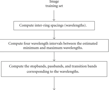
Compute four wavelength intervals between the estimated minimum and maximum wavelengths.

Compute the stopbands, passbands, and transition bands corresponding to the wavelengths.

Compute inter-ring spacings (wavelengths). Image

training set

Figure 4: Filterbank specification from image training set. For uniform wavelength spacing design, the four passbands are set equal to 1/4th of the spacing between the minimum frequency (maximum wavelength) and the maximum frequency (minimum wavelength). For variable frequency spacing, we look at the distribution of the interring spacings in the training set. The basic idea is to search for three jumps (edges) in the interring spacing histogram. Starting from the minimum frequency we select the first interval to the first jump (edge), and so forth, until the maximum frequency.

2. Methods

2.1. Modeling Tree Growth Using an AM-FM Representation. From the introduction, recall that the vascular system of diﬀuse-porous trees such as maple, birch, beech, and aspen is characterized by vessels produced at regular intervals during the growing season and spread evenly throughout the sapwood [1–3]. This leads to the assumption that growth is uniform with respect to the phase. The basicmodel presented here is also closely related to previous AM-FM representation models in [16–18].

We begin with a review of the AM-FM model developed in [16–18]. The tree image is modeled as (section 2 in [16])

Ix,y=ax,yfφ1

x,y,φ2

x,y, (3)

where a(x,y) is a slowly-varying amplitude that is used to capture variations in the minima and maxima of the image, and (x,y)→(φ1(x,y),φ2(x,y)) denotes a curvilinear

coordinate system applied to a periodic function f. Here, φ1(x,y) is aligned with the ridges whileφ2(x,y) is aligned

with the model image equi-intensity lines. In other words, I(x,y)/a(x,y) remains approximately constant along theφ2

-coordinate. We have

fφ1

x,y,φ2

x,y= fφ1

x,y (4)

by abuse of notation. For tree images in the current paper, we note thatφ1(x,y) only changes along the radial direction. In

the discussion that follows, we will drop the subscript from φ1(x,y).

To demonstrate the model, refer to Figure 3. The 1D image profiles of Figure 3refer to image intensity changes

Compute FM function

exp (jφ^)

Estimate derivative using S-G filtering

Estimate IF by dividing derivative by FM function and multiply the

answer by−j.

Extract radial line through the

true image ^ φ

Figure 5: Instantaneous frequency magnitude estimation along the radial direction. For robust estimation, we use an S-G filter to estimate the derivative of the FM function. This is used in estimating the instantaneous frequency (IF) (see (9) for details).

along the radial direction. The beginning of the growth season is marked by a dark tree ring. In the AM-FM model, this is captured by the FM requirement for cosφ(x,y)= −1 which gives

φx,y=π+ 2nπ=(2n+ 1)π, (5)

wheren = 1, 2,. . .,M corresponds to the diﬀerent growth seasons. This is illustrated graphically in Figure 3(a). In

Figure 3(a), the valleys denote the end of a growth season and

the beginning of the next growth season.

Clearly, a full season growth is captured by a phase increase of 2π. Since a full growth season is normally associated with a calendar year, we see that a phase change of 2πcorresponds to a full year. Having said this, it is important to note that tree growth is not uniform over actual time. Here, our assumption is one of relatively uniform growth over the growing season (as opposed to the entire calendar year).

For simplicity, we will consider the wrapped phase function restricted to [0, 2π). Thus, for wrapped phase functions, we capture the start of the growth season using φ(x,y) = π. Then, for the first half of the growth season, we require a change from π to 2π. This is illustrated

in Figure 3(b). For a single season, the first half of the

growth season is captured between the two vertical lines

of Figure 3(b). For the remaining seasons, the pixels that

satisfy π ≤ φ < 2π are shown with horizontal red lines

in Figure 3(b). Similarly, for the second half of the tree

(6)

20 40 60 80 50 100 150 200 250 300 350 400 450 500 550

(a) (b) (c) (d) (e) (f)

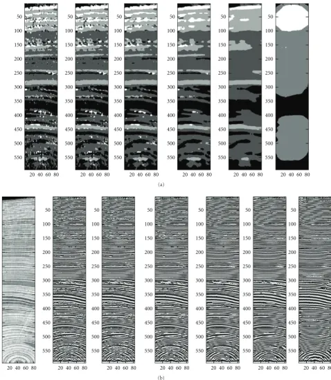
Figure 6: Dominant component analysis example (spruce sample). Left to right: original image, FM output using low frequency filter, FM using medium frequency filter, FM using high frequency filter, FM using very high frequency filter and dominant FM output. Image courtesy: Henry Grissino-Mayer (http://web.utk.edu/∼grissino/Site/gallery/galleries/Tree%20Ring%20Gallery%201/images/ pinaleno%20spruce.jpg).

(iii) 0≤φ < π/2 for the third quarter, and (iv)π/2≤φ < π for the fourth quarter.

2.2. Tree Image Growth Analysis System. We present the entire AM-FM analysis system inFigure 2. To describe the process, we begin with the basic multicomponent model given in (1):

Ix,y≈

M

n=1

an

x,ycosφn

x,y. (6)

We then apply the extended 2D Hilbert transform using [20]

IAS

x,y≈Ix,y+jH2D

Ix,y, (7)

where H2Ddenotes the Hilbert transform operator operating along the columns (or rows) of the image. We implement (7) by taking the 2D FFT of the input image and then zeroing out all the 2D vertical frequencies with a negative frequency component and then multiplying the result by a half. We expect that the output will approximate

IAS

x,y≈ M

n=1

an

x,yexpjφn

x,y. (8)

The analytic signal is then processed through a filterbank.

In Figure 2, we present a separate filterbank specification

system that is used to provide parameters for implementing the filterbank (shown in the upper-left part of the figure). Here, we use a training set of 5 representative images to help determine the relevant parameters, as outlined inSection 2.2. The relevant parameters include specifications for the stop-bands, transition stop-bands, and passbands for each one of the four 2D, separable, channel filters.

Since the channel filters are separable, an eﬃcient imple-mentation consists of first filtering along the rows followed by filtering across the columns. To specify the filters, we only need to derive impulse responses for each of the 1D filters. Here, the impulse response for implementing each filter is computed from its piecewise linear approximation [28].

We provide the pseudocode for computing the impulse response of the 1D filters in Pseudocode 1. The band-pass filters are linear phase, one sided and thus complex valued.

InPseudocode 1, we show how the complex filter coeﬃcients

“an”, “bn” are computed based on the specification of the passband and transition bandwidth. Here, we note that the passbands will always be defined for positive vertical frequency components.

(7)

20 40 60 80 50 100 150 200 250 300 350 400 450 500 550

20 40 60 80 50 100 150 200 250 300 350 400 450 500 550 (a)

20 40 60 80 50 100 150 200 250 300 350 400 450 500 550

20 40 60 80 50 100 150 200 250 300 350 400 450 500 550 (b)

Figure7: Median filtering continuity correction: (a) left to right: filter outputs without median filter, using median filters of sizes 3×3, 5×5, 9×9, 19×19, and 69×69. (b) Left to right: original image (spruce sample), FM image with no median filter, FM image with median filters of sizes 3×3, 5×5, 9×9, 19×19, and 69×69. Image courtesy: Henry Grissino-Mayer.

vertical frequency components dominate. To see this, refer

to Figure 1. There are low-frequencies occurring in all

directions in Figure 1(a). However, higher frequencies are clearly dominant in the vertical direction. It is important to recognize that a full filterbank, covering all directions,

will also enhance structural noise. To see this, refer to

Figure 1(c). InFigure 1(c), tree rings are growing upwards.

(8)

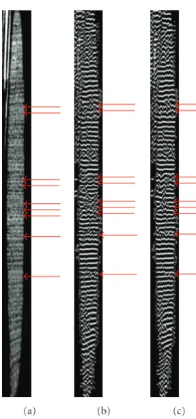
(a) (b) (c)

Figure8: DCA Comparison example (populus sample): (a) original image. (b) FM image without median filter. (c) FM image with median filter correction (69×69). The red arrows indicate the image regions where the median filter correction has significantly improved the continuity in the reconstructed ring.

be rejected. This leads to a great reduction in the number of filters that need to be considered. Empirically, it was determined that no more than 4 filters are needed, (i.e., 4 total channels).

In what follows, we model the output of each channel filter using a single AM-FM component [20]. In other words, we assume thatIAS(x,y)∗ti(x,y)≈ai(x,y) exp[jψi(x,y)], whereti represents the impulse response of theith channel filter, andαi(x,y) exp[jψi(x,y)] represents an AM-FM func-tion. We estimate the AM-FM component functions using

αi

x,y≈IAS

x,y∗ti

x,y,

ψi

x,y≈ArgIAS

x,y∗ti

x,y. (9)

Based on the number of channel filters, we have 4 pairs of estimates of the IA and the IP. At each image pixel, we select the channel filter id (1, 2, 3, or 4) that gives the largest IA estimate. This is termed dominant component analysis [20]. In standard dominant component analysis, we would simply select the estimates from this channel filter. Here, we further process the channel filter id’s using a 2D median filter.

The 2D median filter provides local scale continuity by not allowing random changes in the selected channel filter. The impact of this approach is presented in the results, together with a discussion of the choice of an appropriate

median filter. The IA and IP estimates from the filtered channel id’s are then selected for further processing (see

Figure 2). The estimated dominant component

Ix,y=ax,ycosφx,y (10)

estimates the IA and IP of the tree growth model of

Section 2.1[16–18].

2.3. Filterbank Design Specifications. To specify suitable filter banks, we first analyzed tree ring spacings for a small number of representative samples (see Figures2,4). Representative samples were selected so as to reflect the diversity of growth in the database. In particular, we analyzed 5 images with slow, medium, and fast growth.

Ring spacing can vary significantly over the image. Empirically, we have observed that ring spacing tends to decrease with age (see Figures 1, 16). Therefore, for the highest discrete frequency band, the interring spacing between the two last rings (excluding the bark) was used to estimate the minimum spacing. For determining the passband for the lowest frequency band we need to estimate the largest instantaneous wavelengths of interest. This is done by inspecting the interring spacing found in the first rings in each image (chronologically). For the entire dataset, the minimum vertical frequency (frequency spanning from the wood core center to the bark) was set using the minimum from all the training images. Similarly, the maximum vertical frequency was set by taking the maximum of all estimated maxima.

The simplest filterbank design is to set all the passbands equal (see Figure 4). Here, we computed four wavelength intervals uniformly spaced between the estimated minimum and maximum wavelengths. These intervals were then converted to actual frequency domain filters with transition bands of 0.005π. We refer to this approach as theuniform wavelength spacing design.

By allowing the passbands to vary we consider avariable frequency spacing filterbank. This is done by looking for jumps (edges) in the interring spacing histogram. This approach is similar to edge detection. The minima and max-ima interring spacings are converted to passband frequencies. We used 151 coeﬃcients for implementing the digital filters.

2.4. Instantaneous Frequency Using 1D Savitzky-Golay (S-G) Filtering. We provide a robust method for estimating the instantaneous frequency magnitude along the radial direction. As summarized in Figures2 and 5, we first use the instantaneous phase estimate to form the FM function. We then extract the FM image along the radial line through the center of the tree image. Here, we note that the radial line runs vertically along a column of the image. Thus, no interpolation is required for extracting this column line of pixels. To obtain the central column, we simply take the midpoint column of the image. The midpoint is computed based on the number of pixels in each row of the image.

(9)

50

100

150

200

250

300

350

400

450

500

550

(a) (b)

Figure9: Instantaneous frequency density lines depicted in diﬀerent portions of the FM image. (a) The original spruce image sample. (b) The FM subimage corresponding to row pixels 517–590 of the original image.

20

40

60

80

100

120

140

160

(a)

20

40

60

80

100

120

140

160

(b)

20

40

60

80

100

120

140

160

(c)

20

40

60

80

100

120

140

160

(d)

(10)

(a) Origi-nal

(b) Ground Truth

(c) FM

Figure 11: Results using uniform wavelength spacing filterbank specifications for a Populus sample: (a) original image, (b) manually segmented ground truth, (c) FM image after application of uniform spacing filterbank. The ground truth for this sample is 79 rings.

describe the procedure. First, we express the FM function in terms of its real and imaginary parts:

expjφ(_r)=cosφ(_r) +_jsinφ(_r)_. (11)

In what follows, suppose that we are estimating the radial derivative at r = r0 for the real part of the FM image.

The derivative for the imaginary part is computed in a very similar way. Locally, centered at r = r0, define the

least-squares optimization problem of fitting an nth order polynomial into 2m+ 1> npoints using

Min b

t=m

t=−m

fb(t)−cos

φ(r0+t) 2

, (12)

where the local polynomial of degree is defined by

fb(t)= k=n

k=0

bnktk. (13)

Here, the basic idea is that the polynomial fit estimates the signal while rejecting additive gaussian noise [31]. It relies on the fact that polynomials can be used to approximate continuous and continuously diﬀerentiable functions. Then,

we can estimate the derivative of the FM function atr=r0by

simply evaluating the derivative of fitted polynomial att=0:

∇rcos

φ(r0)

≈dfb

dt(t=0)≈bn1. (14)

Thus, the derivative estimate at every pixel only requires that we estimate bn1. This is accomplished very eﬀectively

by simple convolution with integer Savitzky-Golay (S-G) filter coeﬃcients [31]. In our case, we consider a 2nd order polynomial fit over 9 pixels (n=2,m=4). For computing the derivative, we use

∇rexp

jφ(r0)

≈expjφ(r0)

∗d, (15)

where the derivative convolution kernel is

d= 1

60

4 3 2 1 0 −1 −2 −3 −4, d(0)=0,

(16)

and is applied to both the real and imaginary parts of the FM function.

The IF along the radial direction is then given by

∇rϕ≈ −j

∇rexp

jφ

expjφ . (17)

2.5. Tree Datasets. Twenty tree core samples harvested from native aspen (populus) trees in Colorado were scanned using a MicroCAT II scanner (Imtek, now Siemens, Knoxville, TN). Raw CT attenuation data obtained from each scan was reconstructed at 108μm image voxel resolution using commercially available X-ray CT 2D slice reconstruction software (COBRA, Exxim Corp, Alameda CA). The planar reconstruction images were then loaded and viewed using Amira [32]. The planar projection image that best captured the full tree ring information was selected and saved for further analysis.

For further testing, we also consider a mixture of 12 tree image samples of various types from the Grissino-Mayer database (http://web.utk.edu/∼grissino/). The 12 samples consisted of the following types of trees: bristlecone pine, zuni douglas, avalanche scarred spruce, dominican pine, ponderosa pine, basswood, delaware hemlock, small table mountain pine, sugar maple, foy pine, hemlock, and spruce.

3. Results

3.1. Chirp Image Example Using a Uniform Spacing Filterbank. We use a chirp image to demonstrate the robustness of S-G filtering. The test input image is given by a chirp image expressed as (seeFigure 10(a))

Ix,y=cosφx,y+n1

x,y+n2

x,y, (18)

where n1(x,y) and n2(x,y) are additive Gaussian noise of

(11)

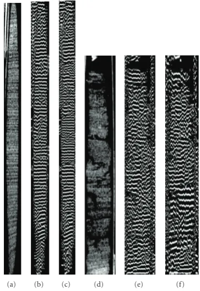
(a) (b) (c) (d) (e) (f)

Figure12: Examples of best and worst result samples for diﬀerent filterbank specifications. Best FM for uniform spacing filterbank results are presented in (a) to (c). (a) Original image. (b) FM image using variable frequency filterbank. (c) FM image using uniform spacing filterbank. The variable frequency spacing filterbank gave a 1.27% error and the uniform spacing filterbank gave a 0% error, meaning it detected all 79 rings. Worst FM for uniform spacing filterbank results are presented in (d) to (f). (d) Original image (2nd example). (e) FM image using variable frequency spacing filterbank (f) and uniform wavelength spacing filterbank. In this second example, the variable frequency spacing filterbank gave a 2.17% error and the uniform spacing filterbank gave a 13% error, meaning it detected only 40 out of 46 rings.

InFigure 10the original chirp image, its noisy version,

the uniform spacing FM reconstruction, and the Structural Similarity Index of the error (SSIM) [33] are presented. The mean SSIM, which measures the image quality based on structural information in the image, was found to be 0.90. This experiment demonstrated the advantages of using the new approach on the basis of improving continuity in the input image.

3.2. Filterbank Design Specification Using Variable Frequency Spacing. We present results for training sets of (i) a single spruce image and (ii) 5 populus image samples. The variable frequency filterbank specifications are given in Table 1 for the 20 populus image, and for the spruce images inTable 2. For both filterbanks, 45 filter coeﬃcients were used. The stopbands, passbands, and transition bands are presented.

For the spruce image (Figure 6), the minimum spacing estimate was 2 pixels and the maximum 13 pixels (unknown resolution). Therefore, the minimum frequency was set at 0.14π and the maximum at 0.98π. A fixed transition width was used for the spruce image. The transition widths for the populus images were varied. In particular, a larger transition band was used for the “very high frequency” channel filter. The populus images were sampled at 106 microns.

Table1: Variable frequency spacing filterbank specifications. The vertical filter parameters for the four filters in the filterbank for the 20 populus images are given in the table. Here, the training set was 5 images and transition bands were set to 0.005. The row filter stopband was set from−0.65 to 0.45 with 0.2 transition bands. All separable filters used 45 coeﬃcients.

Filter Passband Interring spacing in pixels Low frequency 0.15π–0.25π 8.00–13.33 Medium frequency 0.25π-0.26π 7.69–8.00 High frequency 0.26π–0.28π 7.14–7.69 Very high frequency 0.28π–0.30π 6.66–7.14

(12)

10203040 20

40

60

80

100

120

140

160

(a)

0 20 40 60 80 100 120 140 160 180

Pixels −4

−3 −2 −1 0 1 2 3 4

In

stantaneous

p

hase

(b)

0 20 40 60 80 100 120 140 160 180

Pixels

Instantaneous

fr

equency

0.2 0.4 0.6 0.8 1 1.2 1.4 1.6 1.8 2

(c)

Figure13: Radial instantaneous frequency magnitude estimation example (vertical) on noise-free chirp image: (a)–(c). Instantaneous frequency estimation based on S-G filter derivative method: (a) chirp image, (b) instantaneous phase calculated after application of uniform wavelength spacing-based uniform spacing filterbanks. (c) Comparison of estimated radial (vertical) IF magnitude (red) versus ground truth IF (black) for the chirp image. The discrete radial frequency magnitude is expressed in radians.

Table2: Variable frequency spacing specifications for the spruce images. The vertical filter parameters for the four filters are given in the table. Horizontally, for the row filter, the left stopband was from –πto−0.85π, the passband went from−0.65πto 0.45πwith the right stopband from 0.65π toπ. All separable filters used 45 coeﬃcients.

Filter

Low-frequency stopband

Passband

High-frequency

stopband

Interring spacing in

pixels Low

frequency 0–0.14π 0.16π–0.30π 0.32π–π 6.67–12.50 Medium

frequency 0–0.28π 0.30π–0.50π 0.52π–π 4.00–6.67 High

frequency 0–0.48π 0.50π–0.70π 0.72π–π 2.94–4.00 Very high

frequency 0–0.63π 0.70π–0.91π 0.98π–π 2.19–2.94

suﬃcient bandwidth to capture the early ring structure. The vertical filter parameters are summarized inTable 2.

The use of the filterbank for estimating the FM images is demonstrated inFigure 7. InTable 2, we define low, medium, high, and very high frequency components. Clearly, the low frequency components corresponded to the bottom half of the image where there are larger spacings between the rings. Similarly, the medium frequency filter operated right above the middle part of the image. It can be seen that the medium-frequency filter overestimated the number of rings in the lower part of the image. However, over this region, the low-frequency filter produced higher instantaneous amplitude and thus dominated the outputs of all other filters. Similarly, high and very-high frequency components dominated the upper part of the image.

For the populus samples, we used a training set of five images. We provide the results inTable 1.

(13)

−4 −2 0 2 4

0 100 200 300 400 500 600 700

Pixels

0 100 200 300 400 500 600 700

Pixels

Instantaneous

p

hase

0 0.2 0.4 0.6 0.8

Instantaneous

fr

equency

(a)

−4 −2 0 2 4

0 100 200 300 400 500 600 700

Pixels

0 100 200 300 400 500 600 700

Pixels

Instantaneous

phase

0 0.2 0.4 0.6 0.8

In

stantaneous

fr

equency

(b)

Figure14: Radial instantaneous phase and instantaneous frequency magnitude using (a) variable frequency spacing method, and (b) uniform wavelength spacing method. The input image is the populus sample of Figure 12(a). The example shows strong IF magnitude variation.

3.3. FM Image Continuity Improvement Using Dominant Component Analysis and Median Filtering. The use of dom-inant component analysis is summarized in Figures6and7.

InFigure 6, we demonstrate how the individual FM analysis

outputs were combined into the dominant FM image shown on the right. Here, at every pixel, the dominant FM image used the outputs from the filter that produced the largest instantaneous amplitude.

In Figure 7(a) the spatial distribution of the dominant

filters is shown. In Figure 7(a), black denotes the low-frequency filter, while white denotes the highest low-frequency filter. After a careful examination of the input image, it was clear that the second left most image of Figure 7(b) appeared to be noisy. Here, there were rapid changes in the selected dominant filter. To reduce these impulsive changes and support more continuity in the estimates, median filters (with mirror extensions at the edges) of several sizes were

Table3: The relationship between grade and score for the populus samples.

Number of

discontinuities Grade Score

1–4 Excellent 5

5–8 Good 4

9–12 Average 3

13–16 Bad 2

16–20 Very bad 1

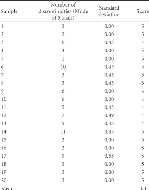
Table4: Tree growth model quality scores for the twenty populus samples. Here, the variable frequency spacing filterbank was used (seeTable 2for the parameters).

Sample

Number of discontinuities (Mode

of 5 trials)

Standard

deviation Score

1 3 0.00 5

2 2 0.00 5

3 6 0.45 4

4 3 0.00 5

5 1 0.00 5

6 10 0.45 3

7 3 0.45 5

8 3 0.45 5

9 6 0.00 4

10 6 0.00 4

11 5 0.45 4

12 7 0.89 4

13 5 0.45 4

14 11 0.45 3

15 2 0.00 5

16 2 0.00 5

17 9 0.55 3

18 3 0.00 5

19 3 0.00 5

20 3 0.00 5

Mean 4.4

used as shown in Figure 7(b). After the application of median filtering, the dominant FM image was recomputed as depicted inFigure 7(b). To determine an appropriate size for the median filter, the resulting FM images ofFigure 7(b) were examined. To evaluate the improvements made by the use of median filtering one comparative example is presented inFigure 8. Arrows are used to illustrate where the improvements are most noticeable.

The instantaneous frequencies (IF) were plotted over the FM image to depict the interring and intraring density flow,

Figure 9(b). The directions of the IF vectors correspond to

(14)

(a) (b) (c)

50

100

150

200

250

300

350

400

450

500

550

(d)

50

100

150

200

250

300

350

400

450

500

550

(e)

50

100

150

200

250

300

350

400

450

500

550

(f)

50

100

150

200

250

300

350

400

450

500

550

(g)

(15)

(a) (b) (c)

50

100

150

200

250

300

350

400

450

500

550

(d)

50

100

150

200

250

300

350

400

450

500

550

(e)

50

100

150

200

250

300

350

400

450

500

550

(f)

50

100

150

200

250

300

350

400

450

500

550

(g)

(16)

(a) (b) (c)

100

200

300

400

500

600

20 40 60 80 100

(d)

20 40 60 80 100 100

200

300

400

500

600

(e)

20 40 60 80 100 100

200

300

400

500

600

(f)

20 40 60 80 100 100

200

300

400

500

600

(g)

(h) (i) (j) (k)

(17)

(a) (b) (c)

100

200

300

400

500

600

(d)

100

200

300

400

500

600

(e)

100

200

300

400

500

600

(f)

100

200

300

400

500

600

(g)

(18)

(f)

(d) (e) (g)

50

100

150

200

250

300

350 50

100

150

200

250

300

350 50

100

150

200

250

300

350 50

100

150

200

250

300

350

Inter-ring discontinuity

Intra-ring

discontinuity

(a) (b)

(c)

(a) (b)

(19)

20

40

60

80

100

120

140

160

180

200

10 20 30

(a)

20

40

60

80

100

120

140

160

180

200

10 20 30

(b)

20

40

60

80

100

120

140

160

180

200

10 20 30

(c)

20

40

60

80

100

120

140

160

180

200

10 20 30

(d)

20

40

60

80

100

120

140

160

180

200

10 20 30

(e)

20

40

60

80

100

120

140

160

180

200

10 20 30

(f)

(20)

Table5: Tree growth model quality scores for the twelve Grissino-Mayer samples. Here, the variable frequency spacing filterbank was used (seeTable 2for the parameters).

Sample

Number of discontinuities (Mode of 5 trials)

Standard

deviation Score

1 6 0.55 4

2 5 0 4

3 3 0 5

4 11 0.55 3

5 7 0.45 4

6 15 0.45 2

7 6 0.45 4

8 10 0.55 3

9 4 0 5

10 3 0 5

11 1 0 5

12 7 0.55 4

Mean 4.0

located. The lengths of the arrows represent the magnitude of ring-density change. As depicted in the IF plots below, the longer arrow lines were oriented towards the bark of the sample, which was the region of greater ring density; that is, more rings per unit length. The reverse relationship was observed for the shorter arrow lines that were oriented towards the pith (center) of the sample where there was lower ring density.

3.4. Tree Image Analysis Example Using a Uniform Spacing Filterbank. A comparative example for a populus (aspen) tree core image is presented in Figure 11. The FM images obtained using the uniform spacing filterbank method is compared with the results of the corresponding images produced without using a filterbank. It is clear that the uniform spacing filterbank method produced a visually improved FM image. The improvements were prominent for both the lower part of the image as well as in the upper-left regions. Here, the minimum frequency for the populus sample was set at 0.12π and the maximum frequency at 0.44π. The filter passbands were 0.12π–0.15π, 0.15π–0.19π, 0.19π–0.27π, and 0.27π–0.44π. Based on the average of all the samples investigated, the minimum passband frequency was 0.01πand the maximum at 0.48π.

3.5. Comparison between Variable Frequency Spacing and Uniform Spacing Filterbanks. In this section a compara-tive example between the uniform spacing filterbank and the fixed-filterbank (variable frequency spacing filterbank) methods is presented. The filterbank changes aﬀected by the uniform spacing filterbank method are also presented.

The best and worst results as judged by the ability to detect the rings on the FM images are depicted inFigure 12. Here, in Figures 12(a) and 12(b), the continuity of the input image allowed the uniform spacing filterbank, which

was used with the median filter for continuity correction, to better adapt to the input. On the other hand, the large discontinuities of the input image in Figure 12(d)did not help the uniform spacing filterbank method. Instead, the use of the dominant component analysis method with the variable frequency spacing filterbank was able to better adjust to the discontinuities. For large discontinuities, the median filtering continuity correction should be carefully verified. InFigure 12(b), we can see that the uniform spacing method also rejected the noisy variations that appeared between rings.

3.6. Radial Instantaneous Frequency Magnitude Estimation Using S-G Filter Derivative Method. This new method was tested on a chirp image after calculating the instantaneous phase from the application of uniform spacing based filter-banks. The results of the test are shown in Figure 13. The instantaneous phase was estimated after the application of uniform spacing-based filter banks. The radial instantaneous frequency magnitude was estimated based on the described method and compared with that from the manually deter-mined ground truth. There is a good match between the estimated IF and ground truth IF magnitudes.

For a populus sample, we present IF results from using both uniform wavelength spacing and variable frequency spacing filterbanks in Figure 14. There appear to be sig-nificant diﬀerence between the two methods. Here, based on visual quality inspection of the output FM images, we found that the variable frequency spacing filterbank gave better results (see discussion below). As shown inFigure 12, the variable frequency spacing filterbank gave significantly improved results for some very diﬃcult cases.

3.7. Tree Growth Estimation. Both the uniform wavelength and the variable frequency filterbanks were used for tree growth estimation. The half-seasonal and quarterly growth estimates are shown in Figure 15 for hemlock, Figure 16 for spruce, Figures 17 and 19 for populus samples using a variable frequency spacing filterbank, and Figure 18 for populus using a uniform wavelength spacing filterbank.

(21)

17, and18are samples with an “excellent” grade. A “good” grade was given if there were between 5 to 8 discontinuities. The “average” score was given if there were between 9 to 12 discontinuities. The example shown in Figure 17was a sample with “average” grade.

The intra- and interring discontinuities are elucidated for this example. The “bad” and “very bad” grade was given if the samples had between 13 to 16 and 17–20 discontinuities, respectively. Table 3 shows the relationship between the criteria for the number of discontinuities, grade, and score.

Table 4presents the number of discontinuities (mode of five

trials) for each populus sample along with the corresponding standard deviation, the graded individual score, and the final average score of all samples. The average score for all 20 samples was 4.4 on a scale of 5.0. Thus, we found that the average results were graded as good to excellent. The same growth modeling study was performed on 12 samples from the Grissino-Mayer database (examples shown in Figures15, 16, and 20). It was found that the average score for the 12 samples was 4.0 on a scale of 5.0 (seeTable 5).

4. Conclusions

From the results we conclude that the use of a variable frequency spacing filterbank provided quality FM images. Furthermore, the continuity of the FM images can be enhanced using median filtering provided that the input image exhibits a reasonable level of continuity as determined by qualitative observation, that is, for images with good and excellent grade (1–8 discontinuities). In this case, the resulting instantaneous frequency vector field characterizes the interring density throughout the wood core sample.

The instantaneous phase allowed us to develop an eﬀ ec-tive growth model. Quarterly and half-seasonal tree growth estimation models were developed and demonstrated. The presented model does provide us with a means for deriving growth estimates from very noisy tree images. The average score based on qualitative criteria using quantitative grading of the 20 populus samples was 4.4 on a scale of 5.0, ranging from good to excellent. Independent testing on a mixture of diﬀerent tree types from the 12 Grissino-Mayer samples gave an average grade of 4.0/5.0. In future work it will be interesting to develop hybrid methods where the results of image analysis are combined with standard measurements such as the tree ring count, tree height, and girth of trunk.

Acknowledgments

The authors would like to especially thank Gerald Tuskan for his useful inputs. This work was partially supported by the BioEnergy Science Center at ORNL; the BioEnergy Science Center is a U.S. Department of Energy Bioenergy Research Center supported by the Oﬃce of Biological and Environmental Research in the DOE Oﬃce of Science. Research was sponsored by the U.S. Department of Energy under contract DE-AC05-00OR22725 with the Oak Ridge National Laboratory, managed by UT-Battelle, LLC. The submitted manuscript has been authored by a contractor

of the U.S. Government under contract no. DE-AC05-00OR22725. Accordingly, the U.S. Government retains a nonexclusive, royalty-free license to publish or reproduce the published form of this contribution, or allow others to do so, for U.S. Government purposes.

References

[1] H. C. Fritts, Tree Rings and Climate, The Blackburn Press, Caldwell, NJ, USA, 1976.

[2] M. K. Hughes, P. M. Kelly, J. R. Pilcher, and V. C. Lamarche Jr., Climate from Tree Rings, Cambridge University Press, Cambridge, UK, 1982.

[3] M. A. Stokes and T. L. Smiley,An Introduction to Tree-Ring Dating, University of Chicago Press, Chicago, Ill, USA, 1968. [4] L. A. Scuderi, “A 2000-year tree ring record of annual

temperatures in the Sierra Nevada mountains,”Science, vol. 259, no. 5100, pp. 1433–1436, 1993.

[5] J. Jiang, X. Gu, and J. Ju, “Significant changes in subseries means and variances in an 8000-year precipitation recon-struction from tree rings in the southwestern USA,”Annales Geophysicae, vol. 25, no. 7, pp. 1519–1530, 2007.

[6] E. R. Cook, D. M. Meko, D. W. Stahle, and M. K. Cleaveland, “Drought reconstructions for the continental United States,”

Journal of Climate, vol. 12, no. 4, pp. 1145–1163, 1999. [7] R. D. D’Arrigo, E. R. Cook, M. E. Mann, and G. C.

Jacoby, “Tree-ring reconstructions of temperature and sea-level pressure variability associated with the warm-season Arctic Oscillation since AD 1650,”Geophysical Research Letters, vol. 30, no. 11, p. 1549, 2003.

[8] A. M. Rae, K. M. Robinson, N. R. Street, and G. Taylor, “Morphological and physiological traits influencing biomass productivity in short-rotation coppice poplar,” Canadian Journal of Forest Research, vol. 34, no. 7, pp. 1488–1498, 2004. [9] G. A. Tuskan, “Short-rotation woody crop supply systems in the United States: what do we know and what do we need to know?”Biomass and Bioenergy, vol. 14, no. 4, pp. 307–315, 1998.

[10] G. Tuskan, D. West, H. D. Bradshaw et al., “Two high-throughput techniques for determining wood properties as part of a molecular genetics analysis of loblolly pine and hybrid poplar,”Applied Biochemistry and Biotechnology, vol. 77, no. 79, pp. 1–11, 1999.

[11] G. A. Tuskan and M. E. Walsh, “Short-rotation woody crop systems, atmospheric carbon dioxide and carbon manage-ment,”Forestry Chronicle, vol. 77, no. 2, pp. 259–264, 2001. [12] G. A. Tuskan, S. P. Difazio, and T. Teichmann, “Poplar

genomics is getting popular: the impact of the poplar genome project on tree research,”Plant Biology, vol. 6, no. 1, pp. 2–4, 2004.

[13] S. D. Wullschleger, T. M. Yin, S. P. DiFazio et al., “Pheno-typic variation in growth and biomass distribution for two advanced-generation pedigrees of hybrid poplar,”Canadian Journal of Forest Research, vol. 35, no. 8, pp. 1779–1789, 2005. [14] W. Larcher, Physiological Plant Ecology, Springer, Berlin,

Germany, 2003.

[15] N. Phillips, R. Oren, and R. Zimmermann, “Radial patterns of xylem sap flow in non-, diﬀuse- and ring-porous tree species,”

(22)

[17] M. S. Pattichis, C. S. Pattichis, M. Avraam, A. C. Bovik, and K. Kyiacou, “AM-FM texture segmentation in electron microscope muscle imaging,”IEEE Transactions on Medical Imaging, vol. 19, no. 12, pp. 1253–1257, 2000.

[18] M. S. Pattichis and A. C. Bovik, “Analyzing image structure by multidimensional frequency modulation,”IEEE Transactions on Pattern Analysis and Machine Intelligence, vol. 29, no. 5, pp. 753–766, 2007.

[19] J. P. Havlicek, D. S. Harding, and A. C. Bovik, “The multicom-ponent AM-FM image representation,”IEEE Transactions on Image Processing, vol. 5, no. 6, pp. 1094–1100, 1996.

[20] J. P. Havlicek, D. S. Harding, and A. C. Bovik, “Multidimen-sional quasi-eigenfunction approximations and multicompo-nent AM-FM models,”IEEE Transactions on Image Processing, vol. 9, no. 2, pp. 227–242, 2000.

[21] V. Murray, P. Rodr´ıguez, and M. S. Pattichis, “Multiscale AM-FM demodulation and image reconstruction methods with improved accuracy,”IEEE Transactions on Image Processing, vol. 19, no. 5, pp. 1138–1152, 2010.

[22] B. J. Super and A. C. Bovik, “Shape from texture using local spectral moments,”IEEE Transactions on Pattern Analysis and Machine Intelligence, vol. 17, no. 4, pp. 333–343, 1995. [23] J. P. Havlicek, J. Tang, S. T. Acton, R. Antonucci, and F. N.

Ouandji, “Modulation domain texture retrieval for cbir in digital libraries,” inProceedings of the Conference Record of the 37th Asilomar Conference on Signals, Systems and Computers, vol. 2, pp. 1580–1584, November 2003.

[24] S. T. Acton, D. P. Mukherjee, J. P. Havlicek, and A. C. Bovik, “Oriented texture completion by AM-FM reaction-diﬀusion,”

IEEE Transactions on Image Processing, vol. 10, no. 6, pp. 885– 896, 2001.

[25] C. Agurto, V. Murray, E. Barriga et al., “Multiscale AM-FM methods for diabetic retinopathy lesion detection,”IEEE Transactions on Medical Imaging, vol. 29, no. 2, pp. 502–512, 2010.

[26] D. J. Fleet and A. D. Jepson, “Computation of component image velocity from local phase information,”International Journal of Computer Vision, vol. 5, no. 1, pp. 77–104, 1990. [27] V. Murray and M. S. Pattichis, “AM-FM demodulation

meth-ods for reconstruction, analysis and motion estimation in video signals,” inProceedings of the IEEE Southwest Symposium on Image Analysis and Interpretation (SSIAI ’08), pp. 17–20, March 2008.

[28] M. S. Pattichis, “Least Squares FIR filter design using fre-quency domain piecewise polynomial approximations,” in

Proceedings of the 10th European Signal Processing Conference, Tampere, Finland, September 2000.

[29] J. Ramachandran, Image analysis of wood core using instan-taneous wavelength and frequency modulation, Ph.D. disserta-tion, The University of New Mexico, 2008.

[30] “The winDendro software,”http://www.regent.qc.ca/products/ dendro/DENDRO.html.

[31] A. Savitzky and M. J. E. Golay, “Smoothing and diﬀerentiation of data by simplified least squares procedures,” Analytical Chemistry, vol. 36, no. 8, pp. 1627–1639, 1964.

[32] “Amira software,”http://www.amira.com.