Volume 2010, Article ID 391798,10pages doi:10.1155/2010/391798
Research Article
Optimization of Weighting Factors for Multiple Window
Spectrogram of Event-Related Potentials
Maria Hansson-Sandsten (EURASIP Member) and Johan Sandberg (EURASIP Member)
Division of Mathematical Statistics, Centre for Mathematical Sciences, Lund University, Box 118, 221 00 Lund, Sweden
Correspondence should be addressed to Maria Hansson-Sandsten,[email protected]
Received 22 December 2009; Accepted 14 May 2010
Academic Editor: Lutfiye Durak
Copyright © 2010 M. Hansson-Sandsten and J. Sandberg. This is an open access article distributed under the Creative Commons Attribution License, which permits unrestricted use, distribution, and reproduction in any medium, provided the original work is properly cited.
This paper concerns the mean square error optimal weighting factors for multiple window spectrogram of different stationary and nonstationary processes. It is well known that the choice of multiple windows is important, but here we show that the weighting of the different multiple window spectrograms in the final average is as important to consider and that the equally averaged spectrogram is not mean square error optimal for non-stationary processes. The cost function for optimization is the normalized mean square error where the normalization factor is the multiple window spectrogram. This means that the unknown weighting factors will be present in the numerator as well as in the denominator. A quasi-Newton algorithm is used for the optimization. The optimization is compared for a number of well-known sets of multiple windows and common weighting factors and the results show that the number and the shape of the windows are important for a small mean square error. Multiple window spectrograms using these optimal weighting factors, from ElectroEncephaloGram data including steady-state visual evoked potentials, are shown as examples.
1. Introduction
Estimation and detection of frequency changes of shorter or longer duration in the ElectroEncephaloGram (EEG) connected to stimuli, for example, evoked or induced potentials are often of great interest. To statistically differ between responses from different types of stimuli, choosing an spectral estimator with small bias and low variance is important.
The idea of multiple windows or multitapering was intro-duced by Thomson, [1], and in the last decades the Thomson method has been used in many different application areas. It has been shown to outperform the Welch method [2] in terms of leakage, resolution, and variance for a stationary spectrally smooth process, [3]. For nonsmooth spectra, however, the performance of the Thomson method degrades due to cross-correlation between subspectra [4]. Other appropriate choices are then, for example, [5–7]. A comparison of Hermite and Slepian functions (the Thomson method) has shown that in the case of time-varying signals
and spectrogram estimation, Hermite functions are a better choice [8].
The choice of windows has been studied in the lit-erature but how to weight the different multiple window spectrograms in the final average has not gained that much attention. In [9], the weighting factors are optimized for the Peak-Matched Multiple Windows, [6]. A criterion is used where normalized bias, variance, and mean square error is optimized for the predefined peaked spectrum. In the nonstationary case, different approaches to approximate a time-varying spectrum with a few windowed spectrograms have been taken, for example, [10–13].
−0.02 0 0.02 0.04 0.06 0.08
100 50
0 0 20 40 60 80
100 120
m
n
(a) Case 1
0 0.02 0.04 0.06 0.08
400 200
0 0 100
200 300
400 500
m
n
(b) Case 2
0 0.02 0.04 0.06 0.08
400 200
0 0 100
200 300
400 500
m
n
(c) Case 3
Figure 1: The three different test covariance matrices for bandlimited white noise processes: (a) stationary process, (b) long-event nonstationary process, and (c) short-event nonstationary process.
denominator. A quasi-Newton algorithm is used for the optimization. We compare the results from the usual equally weighted multiple window spectrogram as well as an optimal scaling factor-adjusted multiple window spectrogram. Pre-liminary results have been presented in [14]. A nonstationary process model, which could be appropriate for, for example, induced responses in the EEG, is studied. We illustrate the weighted multiple window spectrogram estimates by showing examples of steady-state visual evoked potential (SSVEP).
The paper is organized as follows.Section 2presents the optimized weighting factors and inSection 3the evaluation for different stationary and nonstationary processes is pre-sented. In Section 4 examples of estimation of SSVEP are shown.Section 5concludes the paper.
2. Optimization of Weighting Factors
The Multiple Window SpectrogramSx(n,k) of the zero mean
real-valued random processx(n),n=0,. . .,N0−1 is defined
by
Sx(n,k)= I
j=1
αj
N−1
m=0
x(m+nL)hj(m)e−i2π(k/K)m 2
, (1)
fork = 0 · · ·K−1 and 0 ≤n ≤ (N0−N)/L, where the
assumption is that the data is stationary for theN samples x(n L) · · ·x(N−1 +nL). Equation (1) is a weighted sum of spectrograms obtained by using the data windowshj =
[hj(0) · · · hj(N−1)]T, and the weighting factorsαj, j =
1 · · · I. The parameterLis the step size andKthe number of values in the DFT.
With only one window,I =1, the spectrogram has too large variance to be useful in the analysis of a stochastic process, as the variance is approximately the squared Wigner spectrumSx(n,k)2.
2.1. Mean Square Error Optimization. The mean square error
0.124 0.126 0.128 0.13 0.132 0.134 0.136 0.138 0.14
nMSE
TH PM WO HE Methods OPTWEI SCWEI EQWEI (a) Case 1
0.2 0.21 0.22 0.23 0.24 0.25 0.26 0.27 0.28 0.29
nMSE
TH PM WO HE Methods OPTWEI SCWEI EQWEI (b) Case 2
0.1 0.2 0.3 0.4 0.5 0.6 0.7 0.8
nMSE
TH PM WO HE Methods OPTWEI SCWEI EQWEI (c) Case 3
Figure2: The normalized mean square error for the three bandlimited white noise processes with EQWEI (circles), SCWEI (pluses), and OPTWEI (stars) for different window sets, Thomson multiple windows (TH), Peak Matched multiple windows (PM), Welch method (WO), and Hermite functions (HE): (a) stationary process, (b) long-event nonstationary process, and (c) short-event nonstationary process.
The nMSE, which is computed in the time interval [−T·
L· · ·T·L] and in the frequency interval [−M/K· · ·M/K], is the average of a number of (2M+1×2T+1) time-frequency values, giving the cost function:
ξ= 1
(2M+ 1)(2T+ 1)
T
n=−T M
k=−M
ε(n,k)
E2Sx(n,k), (2)
where the MSE for each time and frequency value is defined as
ε(n,k)=VarianceSx(n,k)
+ Bias2S x(n,k)
. (3)
The variance is
VarianceSx(n,k)
=
I
j=1 I
g=1
αjαgcov
Sj(n,k),Sg(n,k)
≈
I
j=1 I
g=1
αjαghTjΦH(k)RnXΦ(k)hg 2
,
(4)
where the covariance matrix Rn
X = E[xxT] with
x = [x(nL)· · ·x(nL + N − 1)]T and Φ(k) = diag [1e−i2πk/K · · · e−i2π(N−1)k/K] and the superscript H
denotes conjugate transpose, according to [4]. Reduction
of the variance is established if the correlation between the windowed periodogram (subspectra),
Sj(n,k)=
N−1
m=0
x(m+n L)hj(m)e−i2π(k/K)m 2
, (5)
from the windowshjandhg,j /=g, is small for all frequency
valuesk. The bias is
BiasSx(n,k)
=ESx(n,k)
−Sx(n,k)
=
I
j=1
αjhTjΦH(k)RnXΦ(k)hj−Sx(n,k),
(6)
where Sx(n,k) is the known Wigner spectrum of the
model. The optimization cost function of (2) includes the expressions of (4) and (6) wherehj, j =1,. . .,I are known
windows andRnX is the time-variable nonstationary
covari-ance matrix. The unknown variables are αj, j = 1,. . .,I
0.12 0.13 0.14 0.15 0.16 0.17 0.18
αj
0 2 4 6 8
j TH PM
WO HE (a) Case 1
0.1 0.15 0.2 0.25 0.3
αj
0 2 4 6 8
j TH PM
WO HE (b) Case 2
0.15 0.2 0.25 0.3 0.35
αj
0 2 4 6 8
j TH PM
WO HE (c) Case 3
Figure3: The optimized weighting factors for the bandlimited white noise process when the different multiple window sets are applied to the different cases, Thomson windows (stars), Peak Matched multiple windows (pluses), Welch method (circles), Hermite functions (crosses): (a) stationary process, (b) long-event nonstationary process, and (c) short-event nonstationary process.
2.2. Averaging and Scale Optimization. Usually, the
spec-trograms from different windows are equally weighted and averaged in the final estimate, that is,
αj=1
I, j=1· · ·I. (7) Using equal weights according to (7) is referred to as equal weights (EQWEI).
The mean square error could be optimized according to the nMSE criterion, using equal weights scaled with a constant factor, that is,
αcj=
c
I, j=1· · ·I, (8) where a closed form expression for the factorcis found from
c=
T n=−T
M
k=−MS2x(n,k)/E2
Sx(n,k)
T n=−T
M
k=−MSx(n,k)/E
Sx(n,k)
. (9)
The weighting factors αc
j are referred to as scaled weights
(SCWEI).
3. Results
3.1. Bandlimited White Noise Process. The evaluation is
done for different stationary and nonstationary processes.
The bandlimited white noise process with the covariance function
rw(n−m)=B
sin(πB(n−m))
πB(n−m) (10) generates a Toeplitz covariance matrix Rstat(n,m), which is
shown inFigure 1(a)forB=(8 + 3)/128≈0.0859, (Case 1). The locally stationary process approach [16,17], where the covariance function of a nonstationary process is defined by
rns(n,m)=rw(n−m)e−((n−m)/2Fsc)
2
e−((n+m)/Fsc)2, (11) gives a variable bandlimited spectrum where the time-variable power of the bandlimited white-noise process changes with a Gaussian envelope. Two examples are seen in
Figure 1(b)as a long-event nonstationary process (Fsc=120)
(Case 2) and inFigure 1(c)as a short-event nonstationary process (Fsc=50) (Case 3).
The weighting factors are optimized using four different sets of multiple windows. The Thomson multiple windows (TH) [1] give uncorrelated subspectra and thereby low variance for a stationary white noise process and the window functionshj are given by the eigenvectors of the (N×N)
Toeplitz covariance matrix with elements given by (10) with
B=I+ 3
N , (12)
0 2 4 6 8 10 12
nMSE
TH PM WO HE Methods OPTWEI SCWEI EQWEI (a) Case 1
0.5 1 1.5 2
nMSE
TH PM WO HE Methods OPTWEI SCWEI EQWEI (b) Case 2
0.5 1 1.5 2 2.5 3 3.5
nMSE
TH PM WO HE Methods OPTWEI SCWEI EQWEI (c) Case 3
Figure4: The normalized mean square error for the three bandlimited peaked spectrum processes with EQWEI (circles), SCWEI (pluses), and OPTWEI (stars) for different window sets, Thomson multiple windows (TH), Peak-Matched multiple windows (PM), Welch method (WO) and Hermite functions (HE): (a) stationary process, (b) long-event nonstationary process, and (c) short-event nonstationary process.
The Peak-Matched (PM) multiple windows [6] are designed to give small correlation between subspectra when the spectrum of the stationary process includes peaks and notches. The windows are given by the solution of the generalized eigenvalue problem where the number of windows satisfies (12). Other parameters to be defined are the peak height chosen as C = 20 dB and the sidelobe suppression chosen as K = 30 dB [6]. The number of windows isIand is related to the bandwidthBand window lengthNas in (12).
The Welch method (WO) [2] utilizes time-shifted equal windows. In this paper we use a Hanning window of appropriate length so that the number of windows,I, is fitted into the total window lengthNwith 50% overlap.
A set of Hermite functions (HE) is computed as
h1(t)=e−t
2/2 ,
h2(t)=2te−t
2/2 ,
hj(t)=2thj−1(t)−2
j−2 hj−2(t), j=3· · · I,
(13)
witht=n/FHforn= −N/2· · ·N/2−1. The parameterFH
is chosen so that the first Hermite function is approximately equal to the first Slepian function of the Thomson method in each case (similar approach as in [8]).
The number of windows is chosen as I = 8 for all different methods and the window lengths are in all cases N = 128 giving B ≈ 0.0859 for the Thomson and Peak-Matched multiple windows. For Case 1 (stationary process), the nMSE is computed and optimized only for the frequency, f = 0, that is, M = 0 and T = 0. For the nonstationary cases we choose, M = 8 and T ·L = 192 withT = 8, (17×17 values) for Case 2 and T·L = 32 with T = 8, (17×17 values) for Case 3. These choices include the whole covariance matrix in each case and give a balance between different time and frequency values in the average.
0 1 2 3 4 5
αj
0 5 10
j TH PM
WO HE (a) Case 1
0 0.1 0.2 0.3 0.4 0.5 0.6
αj
0 2 4 6 8
j TH PM
WO HE (b) Case 2
0 0.1 0.2 0.3 0.4 0.5 0.6
αj
0 2 4 6 8
j TH PM
WO HE (c) Case 3
Figure5: The optimized weighting factors for the bandlimited peaked spectrum process when the different multiple window sets are applied to the different cases, and Thomson windows (stars), Peak Matched multiple windows (pluses), Welch method (circles), and Hermite functions (crosses): (a) stationary process, (b) long-event nonstationary process, and (c) short-event nonstationary process.
able to reach the same nMSE even when the weighting factors are optimized.
In Case 2,Figure 2(b), the results from the long-event nonstationary process show the importance of using SCWEI and OPTWEI compared to the EQWEI in the nonstationary case. The difference of these two sets of weights is, however, not that large. It could also be noted that the Hermite functions perform slightly better than the Thomson multiple windows, which is in concordance with the study of nonsta-tionary processes in [8]. In Case 3,Figure 2(c), using EQWEI on the short-event nonstationary process gives a very large error. Using SCWEI and OPTWEI gives a much lower nMSE. The weighting factors αj for OPTWEI are depicted in
Figure 3for the different window sets and the different cases. For the stationary process, the optimal weighting factors for the Thomson multiple windows (stars) are equally given by αj = 1/8 ≈ 0.125. This is almost also the case for
the Hermite functions (crosses), where the Peak-Matched multiple windows as well as the Welch method give more irregular weighting factors. Overall, however, the optimal weighting factors result almost in equally averaged spectra in all cases which coincides with theory for stationary processes. Of more interest is the long-event nonstationary process in
Figure 3(b), where now both the Thomson and the Hermite windows give weights where more power is given to the spectrogram from the first window function with decreasing power to the following ones. Similar appearance is seen
for the Welch method, where we should remember that all the windows have the same frequency shape but have their power centered at different time points. Most of the power is laid on the resulting spectrograms of the middle windows which intuitively seems quite natural. For the more short-event nonstationary process, the resulting weighting factors have a different behavior, seeFigure 3(c), where now the multiple windows located at end points of the time interval for the Welch method are given most power. This shows the importance of considering the weighting factors in estimation procedure. However, for the bandlimited white noise process, we should remember that using SCWEI in all cases gave almost as small error as OPTWEI.
As the optimization is made using a quasi-Newton algorithm, we cannot be sure of convergence to the global minimum. To verify, we optimize the weighting factors in all cases using 100 different initial sets of weighting factors. The set of initial values is randomly picked from a rectangle distribution with values between zero and one and the resulting sum is normalized to one. For all three bandlimited white noise processes and for all sets of windows, the optimization converged to the same minimum error for all the 100 cases, based on equal sets of weighting factors.
3.2. Bandlimited Peaked Spectrum Process. Instead of using
9 10 11 12 13 14 15 16
F
requency
(Hz)
2 4 6 8 10 12
Time (s) (a) Ex. 1, Hanning
9 10 11 12 13 14 15 16
F
requency
(Hz)
2 4 6 8 10 12
Time (s) (b) Ex. 1 EQWEI/SCWEI
9 10 11 12 13 14 15 16
F
requency
(Hz)
2 4 6 8 10 12
Time (s) (c) Ex. 1, OPTWEI
10 12 14 16 18 20
Fre
q
u
en
cy
(H
z)
2 4 6 8 10 12
Time (s) (d) Ex. 2, Hanning
10 12 14 16 18 20
Fre
q
u
en
cy
(H
z)
2 4 6 8 10 12
Time (s) (e) Ex. 2, EQWEI/SCWEI
10 12 14 16 18 20
Fre
q
u
en
cy
(H
z)
2 4 6 8 10 12
Time (s) (f) Ex. 2, OPTWEI
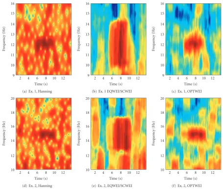
Figure6: Logarithmic spectrogram of SSVEP of long-event nonstationary character, estimated using a single window spectrogram with a Hanning window and the Peak-Matched multiple windows with EQWEI/SCWEI and with OPTWEI fromFigure 5(b). Horizontal and vertical lines indicate flickering light of (a), (b), (c) 12 Hz, 5–10 s, (d), (e),(f) 15 Hz, 5–10 s.
rx(n−m) of a bandlimited peaked spectrum according to
[6]:
Sx
f =
⎧ ⎪ ⎪ ⎨ ⎪ ⎪ ⎩
e−2C|f|/10Blog10(e), f≤B 2,
0, f>B
2.
(14)
In (14), Sx(f) is a peaked spectrum withSx(0) = 1,B =
11/128≈0.0859, andSx(B/2)= −CdB, whereC = 20 dB.
The nonstationary processes are found from (11) withrw(n−
m) replaced withrx(n−m).
The results from these processes are presented in
Figure 4. For the stationary-peaked spectrum process,
Figure 4(a), the EQWEI of the Welch method happens to give the smallest error. Using SCWEI we can lower the nMSE for all methods but using OPTWEI combined with Peak Matched multiple windows gives the smallest nMSE of all methods, which is concordance with [6, 9], where these windows and optimized weighting factors are shown to be
optimal for this process. In Case 2,Figure 4(b), for the long-event nonstationary process, the benefit of using windows with properties suitable for the process becomes visible as the smallest nMSE is given for the Peak-Matched multiple windows combined with OPTWEI. In this case, the SCWEI is far from giving the same result. In Case 3, we also see a similar result for the short-event nonstationary process.
The different weighting factors are depicted inFigure 5, and for the stationary case, we see in Figure 5(a) the characteristic weighting for the PM given by 1/λi, whereλiis
6 8 10 12
F
requency
(Hz)
8 10 12 14
Time (s) (a) Ex. 3, Hanning
6 8 10 12
F
requency
(Hz)
8 10 12 14
Time (s) (b) Ex. 3, EQWEI/SCWEI
6 8 10 12
F
requency
(Hz)
8 10 12 14
Time (s) (c) Ex. 3, OPTWEI
6 8 10 12 14
Fre
q
u
en
cy
(H
z)
2 4 6 8
Time (s) (d) Ex. 4, Hanning
6 8 10 12 14
Fre
q
u
en
cy
(H
z)
2 4 6 8
Time (s) (e) Ex. 4, EQWEI/SCWEI
6 8 10 12 14
Fre
q
u
en
cy
(H
z)
2 4 6 8
Time (s) (f) Ex. 4, OPTWEI
Figure7: Logarithmic spectrogram of SSVEP of short-event nonstationary character, estimated using a single window spectrogram with a Hanning window and the Peak-Matched multiple windows with EQWEI/SCWEI and with OPTWEI fromFigure 5(b). Horizontal and vertical lines indicate flickering light of (a), (b), (c) 9 Hz, 10.4–12.2 s, (d), (e), (f) 9 Hz, 4.7–5.7 s.
the peaked spectrum process and the bandlimited white noise process and also how the weighting changes with the non-stationarity of the process.
The convergence of the optimization of the weighting factors in the three cases of bandlimited peaked spectrum processes is also investigated using the same randomly picked initial values as for the bandlimited white noise process and all different window sets. The results show that a minimum of 90% (usually around 95%) of the initial values converge to the global minimum giving the true optimal weighting factors. In the cases where the algorithm did not converge, the final error and the weighting factors were very far away from the true values and the divergence was easily discovered.
4. Real Data Examples
To show the performance for real-data, sampled ElectroEn-cephaloGram data (EEG) were studied, where a flickering light (Grass Photic stimulator Model PS22C) was introduced
at different time points. The light stimulation lasted approx-imately 1 s or 5 s. For a repetitive periodic visual stimulus a steady-state visual evoked potential (SSVEP) arises in the EEG. We assume the short stimulation (∼1 s) to introduce a short-event nonstationary process and the long stimulation (∼5 s) to introduce a long-event nonstationary process in the measured EEG. The subject was supine with closed eyes on a bed in a silent laboratory where ambient light was dimmed. The flickering light, with set frequency and time interval, was flashed at the subject from a distance of approximately 1 m. Data were recorded using a Neuroscan system with a digital amplifier (SYNAMP 5080, Neuro Scan, Inc.). Amplifier band-pass settings were 0.3 and 50 Hz. The sample rate was 256 Hz which was downsampled to a sample rate ofFs=64 Hz in Matlab. In all examples channel PZ is
chosen.
the flickering lasts between time points 5 and 10 s and we assume these responses to be two long-event nonstationary processes. The third and fourth examples are given from flickering of 9 Hz between time points 10.4 and 12.2 s and time points 4.7 and 5.7 s, respectively. These two examples are assumed to be responses of short-event nonstationary processes.
We assume that we can model the different long-event nonstationary SSVEPs of Examples 1 and 2 as ban-dlimited peaked spectrum processes; see [18]. Logarithmic spectrograms are depicted in Figure 6, where we compare the spectrograms using the single Hanning window with different weightings of the Peak Matched multiple windows using OPTWEI from Figure 5(b) and EQWEI/SCWEI. In all cases, the window length is N = 128. Note that the spectrogram using EQWEI is equal to SCWEI as the difference is only a gain factor and the coloring is adjusted between the minimum and maximum value of each plot. We should also remember that the bandwidth of this estimator isB=Fs(I+ 3)/N =5.5 Hz, which is also clearly seen in the
examples in Figures6(b)and6(e). The spread of the power caused by the large frequency bandwidth makes it difficult to know where the actual response frequency is located. Equal weighting of the multiple window spectrograms is not appropriate for data where it is important to locate the maximum power at a certain frequency. In the time-scale, however, we see that the resulting responses show up in the time interval where they should be located according to the stimuli given. The single window Hanning spectrograms are well resolved in frequency but the variance is however too large to be reliable, which is seen in Figures 6(a) and
6(d).
InFigure 7, we compare the spectrogram estimates using the single Hanning window with different weightings of the Peak-Matched multiple windows using OPTWEI from
Figure 5(c)and EQWEI/SCWEI. The single Hanning spec-trogram in Figures 7(a) and 7(d) is difficult to interpret and the spectrograms using EQWEI/SCWEI give a too wide estimate in frequency; see Figures 7(b) and 7(e). Using OPTWEI, the short-event nonstationary processes in Figures
7(c) and7(f) are located correctly in the time interval as well as at the appropriate frequency. The last case however,
Figure 7(f), has a large amount of power outside the time interval of stimuli, around 6-7 s. This is explained by the fact the stimulus sequence also activated the person and thereby also the alpha activity raised; see [18].
Even better is to actually estimate a model covariance function, using, for example, many trials from the same experiment for a robust estimate. From the properties of this modeled covariance function an appropriate set of multiple windows can be chosen and the weighting factors could be nMSE optimized to estimate the single stimulus response.
5. Conclusion
We compare the Hermite functions, the Thomson windows, the Peak-Matched Multiple Windows, and the Welch win-dows and compute the performance with optimal weighting factors for different stationary and nonstationary processes.
The cost function for optimization is the normalized mean square error where the normalization factor is the multiple window spectrogram. This means that the unknown weight-ing factors will be present in the numerator as well as in the denominator. A quasi-Newton algorithm is used for the optimization. The results show that the weighting factors, as well as the shape of the windows, are important factors for a small error. It is also shown that a scaling optimization of the usual averaging could give almost as small mean square error as an optimization of the individual weighting factors in case of a smooth spectrum. For a peaked spectrum, a significant reduction of the normalized mean square error is achieved using individual optimization of the weights.
Acknowledgment
This paper is supported by the Swedish Research Council.
References
[1] D. J. Thomson, “Spectrum estimation and harmonic analysis,”
Proceedings of the IEEE, vol. 70, no. 9, pp. 1055–1096, 1982. [2] P. D. Welch, “The use of fast fourier transform for the
estima-tion of power spectra: a method based on time averaging over short, modified periodograms,”IEEE Transactions on Audio Electroacoustics, vol. 15, no. 2, pp. 70–73, 1967.
[3] T. P. Bronez, “On the performance advantage of multitaper spectral analysis,”IEEE Transactions on Signal Processing, vol. 40, no. 12, pp. 2941–2946, 1992.
[4] A. T. Walden, E. McCoy, and D. B. Percival, “Variance of multitaper spectrum estimates for real Gaussian processes,”
IEEE Transactions on Signal Processing, vol. 42, no. 2, pp. 479– 482, 1994.
[5] K. S. Riedel and A. Sidorenko, “Minimum bias multiple taper spectral estimation,”IEEE Transactions on Signal Processing, vol. 43, no. 1, pp. 188–195, 1995.
[6] M. Hansson and G. Salomonsson, “A multiple window method for estimation of peaked spectra,”IEEE Transactions on Signal Processing, vol. 45, no. 3, pp. 778–781, 1997. [7] B. Farhang-Boroujeny, “Prolate filters for nonadaptive
multi-taper spectral estimators with high spectral dynamic range,”
IEEE Signal Processing Letters, vol. 15, pp. 457–460, 2008. [8] M. Bayram and R. G. Baraniuk, “Multiple window
time-frequency analysis,” in Proceedings of IEEE-SP International Symposium on Time-Frequency and Time-Scale Analysis, pp. 173–176, June 1996.
[9] M. Hansson, “Optimized weighted averaging of peak matched multiple window spectrum estimates,”IEEE Transactions on Signal Processing, vol. 47, no. 4, pp. 1141–1146, 1999. [10] F. C¸akrak and P. J. Loughlin, “Multiple window time-varying
spectral analysis,”IEEE Transactions on Signal Processing, vol. 49, no. 2, pp. 448–453, 2001.
[11] J. Xiao and P. Flandrin, “Multitaper time-frequency reas-signment for nonstationary spectrum estimation and chirp enhancement,”IEEE Transactions on Signal Processing, vol. 55, no. 6, pp. 2851–2860, 2007.
[12] W. J. Williams and S. Aviyente, “Spectrogram decompositions of time-frequency distributions,” in Proceedings of the 6th International, Symposium on Signal Processing and its Applica-tions (ISSPA ’01), pp. 587–590, 2001.
no. 1, pp. 179–189, 2001.
[14] M. Hansson-Sandsten and J. Sandberg, “Optimization of weighting factors for multiple window time-frequency analy-sis,” inProceedings of the European Signal Processing Conference (EUSIPCO ’09), Glasgow, UK, 2009.
[15] R. Fletcher,Practical Methods for Optimization, John Wiley & Sons, New York, NY, USA, 1987.
[16] R. A. Silverman, “Locally stationary random processes,”IRE Transactions on Information Theory, vol. 3, pp. 182–187, 1957. [17] P. Wahlberg and M. Hansson, “Kernels and multiple windows for estimation of the Wigner-Ville spectrum of Gaussian locally stationary processes,” IEEE Transactions on Signal Processing, vol. 55, no. 1, pp. 73–84, 2007.
[18] M. Hansson and M. Lindgren, “Multiple-window spectro-gram of peaks due to transients in the electroencephalospectro-gram,”