Volume 2006, Article ID 96421, Pages1–19 DOI 10.1155/ASP/2006/96421
Floating-to-Fixed-Point Conversion for Digital
Signal Processors
Daniel Menard, Daniel Chillet, and Olivier Sentieys
R2D2 Team (IRISA), ENSSAT, University of Rennes I, 6 rue de Kerampont, 22300 Lannion, France
Received 1 October 2004; Revised 7 July 2005; Accepted 12 July 2005
Digital signal processing applications are specified with floating-point data types but they are usually implemented in embedded systems with fixed-point arithmetic to minimise cost and power consumption. Thus, methodologies which establish automati-cally the fixed-point specification are required to reduce the application time-to-market. In this paper, a new methodology for the floating-to-fixed point conversion is proposed for software implementations. The aim of our approach is to determine the fixed-point specification which minimises the code execution time for a given accuracy constraint. Compared to previous method-ologies, our approach takes into account the DSP architecture to optimise the fixed-point formats and the floating-to-fixed-point conversion process is coupled with the code generation process. The fixed-point data types and the position of the scaling opera-tions are optimised to reduce the code execution time. To evaluate the fixed-point computation accuracy, an analytical approach is used to reduce the optimisation time compared to the existing methods based on simulation. The methodology stages are de-scribed and several experiment results are presented to underline the efficiency of this approach.
Copyright © 2006 Daniel Menard et al. This is an open access article distributed under the Creative Commons Attribution License, which permits unrestricted use, distribution, and reproduction in any medium, provided the original work is properly cited.
1. INTRODUCTION
Most embedded systems integrate digital signal processing applications. These applications are usually designed with high-level description tools like CoCentric (Synopsys), Mat-lab/Simulink (Mathworks), or SPW (CoWare) to evaluate the application performances with floating-point simula-tions. Nevertheless, if digital signal processing algorithms are specified and designed with floating-point data types, they are finally implemented into fixed-point architectures to sat-isfy the cost and power consumption constraints associated with embedded systems. In fixed-point architectures, mem-ory and bus widths are smaller, leading to a definitively lower cost and power consumption. Moreover, floating-point op-erators are more complex to process the exponent and the mantissa. Thus, floating-point operator area and latency are greater compared to fixed-point operators.
In this context, the application specification must be con-verted into fixed-point. The manual conversion process is a time-consuming and an error-prone task which increases the development time. Some experiments [1] have shown that this manual conversion can represent up to 30% of the global implementation time. To reduce the application time-to-market, high-level development and code genera-tion tools are needed. Thus, methodologies for automatic
floating-to-fixed-point conversion are required to accelerate the development.
For digital signal processors (DSPs), the methodology aim is to define the optimised fixed-point specification which minimises the code execution time and leads to a suffi -cient accuracy. For this accuracy, the desired application per-formances must be reached. Existing methodologies [2,3] achieve a floating-to-fixed-point transformation leading to an ANSI-C code with integer data types. Nevertheless, the data types supported by the DSP and the processor scaling capabilities are not taken into account to determine the fixed-point specification. The analysis of the architecture influence on the computation accuracy underlines the necessity to take the DSP architecture into account to optimise the fixed-point specification [4]. Furthermore, the code generation and the conversion process must be coupled.
and the selection of the data word-length according to the different data types supported by recent DSPs. The scal-ing operations are moved to reduce the code execution time. This paper is organised as follows. The previous works for the floating-to-fixed-point conversion are presented in
Section 2. Our methodology is detailed inSection 3. For the different methodology stages, our approach is justified and the technique used to solve the problem is described. Finally, inSection 4, different experiments are presented underlining the efficiency of our approach.
2. RELATED WORKS
2.1. Floating-to-fixed-point conversion methodologies
In this section the different available methodologies for the automatic implementation of floating-point algorithms into fixed-point architectures are presented.
In [5], a methodology which implements floating-point algorithms into the TMS320C25/50 fixed-floating-point DSP (Texas Instruments) is proposed. The floating-to-fixed-point conversion is achieved after the code generation process. This methodology is specialised for this particular archi-tecture and cannot be transposed to other archiarchi-tecture classes.
The two methodologies presented below achieve the floating-to-fixed-point transformation at the source code level. The FRIDGE [6] methodology, developed at the Aachen University, transforms the floating-point C source code into a C code with fixed-point data types. In the first step, calledannotations, the user defines the fixed-point for-mat of some variables which are critical in the system or for which the fixed-point specification is already known. More-over, global annotations can be defined to specify some rules for the entire system (maximal data word-length, casting rules). The second step, called interpolation [6, 7], deter-mines the application point specification. The fixed-point data formats are obtained from a set of propagation rules and the analysis of the program control flow. This de-scription is simulated to verify if the accuracy constrains are fulfilled. The commercial toolCoCentric Fixed-point Designer proposed by Synopsys is based on this approach.
In [3] a method called embedded approachis proposed to generate an ANSI-C code for a DSP compiler from the fixed-point specification. The data (source data), for which the fixed-point formats have been obtained with the tech-nique presented previously, are specified with the available data types (target data) supported by the target processor. The degrees of freedom due to the source data position in the target data are used to minimise the scaling operations. This methodology produces a bit-true implementation into a DSP of a fixed-point specification. But accuracy and execu-tion time are not optimised through the fixed-point format modification of some relevant variables.
The aim of the tool presented in [2,8] is to transform a floating-point C source code into an ANSI-C code with integer data types. This code is independent of the targeted architecture. Moreover, a fixed-point format optimisation is
done to minimise the number of scaling operations. Firstly, the floating-point data types are replaced by fixed-point data types and the scaling operations are included in the code. The scaling operations and the fixed-point data formats are determined from the dynamic range information obtained with a statistical method [9]. The reduction of the scaling operations number is based on the assignation of a common format to several relevant data to minimise the scaling oper-ations cost function. This cost function takes account of the number of each scaling operation occurrences and depends on the processor scaling capabilities. For a processor with a barrel shifter, the cost of a scaling operation is set to one cy-cle; otherwise the number of cycles required for a shift ofn bits is equal toncycles.
This methodology achieves the floating-to-fixed-point conversion with the minimisation of the scaling operations cost. But, the code execution time is not optimised under a global accuracy constraint. The accuracy constraint is only specified through the definition of a maximal acceptable ac-curacy degradation allowed for each data. The data types supported by the architecture are not taken into account to optimise the fixed-point data formats. Moreover, the archi-tecture model used to minimise the scaling operations num-ber is not realistic. Indeed, for conventional DSPs including a barrel shifter and based on a MAC (multiply-accumulate) structure, the scaling operation execution time depends on the data location in the data path and is not always equal to one cycle. Furthermore, for processors with instruction-level parallelism (ILP) capabilities, the overhead due to scaling op-erations depends on the scheduling step and cannot be easily evaluated before the code generation process.
Compared to these methods, our approach optimises the data word-length to benefit from the different data types sup-ported by recent DSPs. Moreover, the scaling operation loca-tion is optimised with a realistic model to evaluate the scaling operation execution time. The goal of these two optimisa-tions is to minimise the code execution time as long as the accuracy constraint is fulfilled. In our methodology, the pro-cessor architecture is taken into account and the floating-to-fixed-point conversion process is coupled with the code gen-eration process.
2.2. Fixed-point accuracy evaluation
of the fixed-point specification accuracy, a new simulation is required.
An alternative to the simulation-based method is the ana-lytical approach. The verification that the fixed-point imple-mentation respects the application quality criteria is achieved in two steps with the help of a single metric. The most com-monly used metric to evaluate the computation accuracy is the signal-to-quantisation-noise ratio (SQNR) [10,13,14]. This metric defines the ratio between the desired signal power and the quantisation noise power. Thus, first of all, the minimal value of the computation accuracy (SQNRmin) is determined and then, the fixed-point specification is op-timised under this accuracy constraint. The accuracy con-straint (SQNRmin) is determined according to the application performance constraints. The main advantage of the analyt-ical approach is the execution time reduction of the fixed-point optimisation process. Indeed, the SQNR expression de-termination is done only once, then, the fixed-point system accuracy is evaluated through the computation of a mathe-matical expression.
In our methodology, an analytical approach is used to evaluate the computation accuracy. This approach [14] re-duces significantly the execution time of the fixed-point optimisation process, compared to the simulation-based methods. This method is described with further details in
Section 3.1.3.
3. FLOATING-TO-FIXED-POINT CONVERSION
METHODOLOGY
The aim of the methodology presented in this paper is to implement automatically a floating-point application into a fixed-point DSP. Despite the computation error due to the fixed-point arithmetic, the different quality criteria (perfor-mances) associated with the application must be respected. For embedded systems, the cost and the power consumption must be minimised. Thus, the optimised fixed-point specifi-cation which minimises the code execution time and fulfils a given computation accuracy constraint must be determined. To optimise the implementation, the targeted architecture must be taken into account during the fixed-point conver-sion process.
3.1. Methodology flow
The methodology flow has been defined from the analysis of the architecture influence on the computation accuracy and from the study of the interaction between the fixed-point conversion process and the code generation process. The global methodology flow is presented inFigure 1. The tool is made up of two main blocks corresponding to the compilation infrastructure and to the floating-to-fixed-point conversion.
The compilation infrastructure front-end generates an intermediate representation from the floating-point C source code. The floating-to-fixed-point conversion process is ap-plied on this intermediate representation. The assembly code is generated with the compilation infrastructure back-end from this fixed-point intermediate representation.
The first stage of the fixed-point conversion process cor-responds to the data dynamic range evaluation. These re-sults are used to determine the data binary-point position which avoids overflows. Then, the data word-lengths are de-termined to obtain a complete fixed-point specification. The data types which minimise the code execution time and re-spect the accuracy constraint are selected. Finally, the scaling operation locations are optimised to minimise the code exe-cution time as long as the accuracy constraint is fulfilled. This conversion process is achieved under an accuracy constraint to obtain a fixed-point specification which satisfies the appli-cation performances. Thus, the computation accuracy must be evaluated and the accuracy constraint must be determined from application performances.
3.1.1. Compilation infrastructure
The floating-point C source algorithm is transformed into an intermediate representation with the compiler front-end. This intermediate representation (IR) specifies the applica-tion with a control and data flow graph (CDFG). The tool uses the SUIF compiler front-end [15], and the CDFG is generated from SUIF’s internal-representation abstract trees. This CDFG is made up of different control flow graphs (CFGs) and data flow graphs (DFGs). Each CFG represents one of the application control structures. These structures correspond to basic blocks, conditional and repetitive struc-tures. The core of conditional and repetitive structures is specified with a CFG. Each control structure block contains a specification of its input and output data. The basic block represents a set of sequential computations without control structure. The different computations of a basic block core which correspond to the signal processing part are repre-sented with a data flow graph (DFG). The DFG includes the delay operations. To illustrate this intermediate representa-tion, an FIR (finite impulse response) filter example is under consideration. The floating-point C source code is given in
Algorithm 1and the corresponding intermediate representa-tion is presented inFigure 2.
The code generation is achieved with the flexible code generation tool CALIFE presented in [16] and the processor is described with the ARMOR language [17].
3.1.2. Fixed-point format
A fixed-point data is made up of an integer part and a frac-tional part as presented inFigure 3. The fixed-point format of a data is specified as (b,m,n), wherebis the data word-length. The terms mandn are the binary-point positions referenced, respectively, from the most significant bit (MSB) and the least significant bit (LSB). In fixed-point arithmetic, mandnare fixed and lead to an implicit scale factor which stays constant during the processing.
Application performances
Accuracy evaluation
fSQNR(−→b,−→m)
Accuracy constraint determination
SQNRmin
GApp
Dynamic range determination
GDR
Binary-point position determination
GBP
Data type selection
GWL
Scaling operation optimisation
GSO
Floating-to-fixed-point conversion Processor model DSP
description
Processor model generation
CDFG IR C generation
C source code
Compiler front-end
Compiler back-end Code generation
Assembly code
Fixed-point C code or SystemC
C
o
mpilation
infr
ast
ru
ctur
e
Figure1: Methodology flow for the floating-to-fixed-point conversion. The tool is made up of two main blocks corresponding to the compilation infrastructure and to the floating-to-fixed-point conversion.
floath[32]= {−0.0297,. . ., 0.897, 0.98, 0.897,. . .,−0.0297}; floatx[32];
floaty, acc;
float fir (float input)
{
inti;
x[0]=input;
acc=x[0]∗h[0] ;
for (i=31;i >0;i− −)
{
acc=acc +x[i]∗h[i]; x[i]=x[i−1];
}
y=acc;
returny;
}
Algorithm 1: Specification of the 32-tap FIR filter with the floating-point C source code.
and the binary-point positions associated with the oper-ation oi. For a CDFG made up of No operations, −→b = [b1,b2,. . .,bi,. . .,bNo] and m→− = [m1,m2,. . .,mi,. . .,mNo]
are the vectors specifying, respectively, the word-length and the binary-point position of all CDFG operation operands.
CFG FIR B.B. 1
For
B.B. 3
B.B.: basic block
CFG for B.B. 2
Acc =
y DFG
3
Input =
x[0] h[0] ×
DFG 1 Acc
x[i−1] Acc
z−1
x[i] h[i] ×
u
+ DFG 2
Acc
Figure 2: The control and data flow graph equivalent to
Algorithm 1(the nodez−1corresponds to a delay operation).
3.1.3. Computation accuracy management
S bm−1bm−2 b1 b0 b−1 b−2 b−n+2b−n+1b−n
Sign
bit 2m−1 Integer part 20 2−1 Fractional part 2−n
MSB
m n LSB
b
Figure3: Fixed-point data specification:b,m, andnrepresent, re-spectively, the data word-length, the binary-point position refer-enced from the MSB (integer part), and the binary-point position referenced from the LSB (fractional part).
y my
x mx
my
mx Ops.
Operation
mz z
mz
Data
Figure 4: Binary-point position model for an operation. The binary-point position for the operation inputs and output are spec-ified bymx,my, andmz.
Accuracy constraint determination
The accuracy constraint corresponding to the minimal value (SQNRmin) of the SQNR is determined according to the application performance constraints. This SQNR minimal value is obtained with a floating-point simulation of the ap-plication as presented inFigure 5. The error due to the fixed-point conversion is modelled by a noise source (qy) located at the system output. The power of this noise source is in-creased as long as the application performance constraints are respected. The SQNR constraint is determined from the maximal value of the noise source power which ensures that the application performances are still reached.
Computation accuracy evaluation
To determine the SQNR expression, the main challenge cor-responds to the computation of the system output quantisa-tion power. In fixed-point system, a quantisaquantisa-tion noiseqgkis generated when some bits are eliminated during a cast opera-tion. Each quantisation noise sourceqgkis propagated inside the system and contributes to the output quantisation noise qythrough the gainαkas presented inFigure 6. The goal of the analytical approach is to define the power expression of the output noiseqyaccording to theqgknoise source statisti-cal parameters and the gainsαkbetween the output and the different noise sources.
For linear time-invariant systems, each αk term is ob-tained from the transfer function between the system output and theqgk noise source. The transfer functions are deter-mined from the data flow graph [18] representing the appli-cation [14]. They are obtained from theZtransform of the recurrent equations representing the system. The recurrent equations are built by traversing the graph from the inputs to the output. This technique requires that the graph be acyclic.
Floating-point system
Output quantisation noise model
y y
qy
+ Quality criteria verification
max(Pqy) SQNRmin
determination
SQNRmin
Quality criteria
Application
Fixed-point system model
Figure 5: Technique to determine the accuracy constraint. The global error due to the fixed-point conversion is modelled by a noise source (qy).
q0
qi
qN
α0
αi
αN
+ qy
Figure6: Output quantisation noise model in a fixed-point system. The system output noiseqyis a weighted sum of the different noise
sourcesqgk.
Thus, the DFG is transformed into several directed acyclic graphs (DAGs) when cycles are present like in the case of re-cursive1structures.
In nonrecursive2and nonlinear systems, eachα
kterm is obtained from the signals associated with each operation in-volved in theqgk noise source propagation towards the out-put [19]. Theαkterm expressions are built by traversing the acyclic graph from the inputs to the output. The statistical parameters ofαkare determined with a single floating-point simulation.
The qgk noise source statistical parameters are deter-mined from the models presented in [20]. The statistical pa-rameters depend on the number of bits eliminated and the data format after the cast operation. As described in (1), the SQNR is a function of the vector −→b and−→m specified inSection 3.1.2. This function is determined automatically from the data flow graph representing the application with the technique summarised in the previous paragraph and de-tailed in [14,19]:
SQNR= fSQNR(−→b,−→m). (1)
1In a recursive structure, the system output depends on the input samples
and the previous output samples.
2In a nonrecursive structure, the system output depends only on the input
3.1.4. Floating-to-fixed-point conversion
For the floating-to-fixed-point conversion process, the data dynamic range is first evaluated. The results are used to de-termine the binary-point position of each data. Then, the data word-length is selected according to the data types sup-ported by the targeted DSP. Finally, the fixed-point speci-fication is optimised by moving the scaling operations to reduce the code execution time. The data word-length and the scaling operation location are optimised under accuracy constraint. These different transformations in the conversion process lead to the CDFGGDR,GBP,GWL, andGSOand are detailed in the following sections. The optimised fixed-point specification obtained after the conversion process can be transformed into a fixed-point C code or a SystemC code. This code can be used to simulate the fixed-point specifica-tion and to verify that the applicaspecifica-tion quality criteria are re-spected.
3.2. Data dynamic range determination
The first stage of the methodology corresponds to the data dynamic range evaluation. This stage only depends on the application and the input signals. To evaluate an applica-tion data dynamic range, two approaches based on statisti-cal or analytistatisti-cal methods can be used. The dynamic range can be computed from the data statistical parameters which are obtained with a floating-point simulation. The estima-tion results depend on the data used for the simulaestima-tion. This approach produces an accurate estimation of the dynamic range from signal characteristics. It guarantees a low over-flow probability for signals with the same characteristics. Nevertheless, overflows can occur for signals with different statistical properties.
The second class of methods corresponds to the ana-lytical approaches which are based on the computation of the data dynamic range expressions from the input dynamic range. These methods guarantee that no overflow will occur but lead to a more conservative estimation. Indeed, the dy-namic range expression is computed in the worst case. The data dynamic range can be obtained with the interval arith-metic theory [21]. The operation’s output dynamic range is determined from its input dynamic. A worst-case dynamic range propagation rule is defined for each type of opera-tion. Each data dynamic range is obtained with the help of the propagation rules during the application graph traver-sal. Thus, this technique cannot be used in the case of cyclic graphs like in recursive structures.
For linear time-invariant systems, the data dynamic range can be computed from the L1 or Chebyshev norm [22] according to the input signal frequency characteristics. These norms compute the data dynamic range in the case of lin-ear time-invariant systems based on a nonrecursive or re-cursive structure. To evaluate the dynamic range of a data difrom the system inputx, the transfer function of the sub-system with thedioutput and thex input has to be deter-mined.
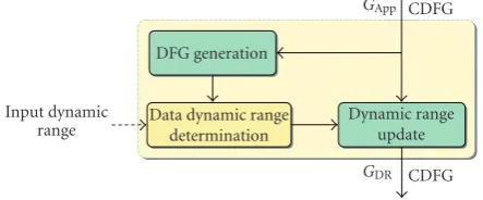
In our methodology, these two analytical approaches have been combined to determine the data dynamic range in
Input dynamic range
DFG generation
Data dynamic range determination
GApp CDFG
Dynamic range update
GDR CDFG
Figure7: Methodology flow for the data dynamic range determi-nation. The dynamic range is computed on the DFG representing the application and then the global CDFG is annotated with the dy-namic range information.
nonrecursive systems and in recursive linear time-invariant systems. The structure of this module is presented in
Figure 7. The module input is the intermediate representa-tion corresponding to the applicarepresenta-tion CDFGGApp. The first step eliminates the control structures of the CDFG to ob-tain a data flow graph (DFG). For repetitive structures, the loops are unrolled, and for conditional structures, the branch which leads to the worst case is retained.
The second step corresponds to the dynamic range com-putation for each data of the application DFG. For nonrecur-sive structures the dynamic range information are obtained by traversing the graph from the sources to the sinks. For each operation, a propagation rule is applied as defined in [21]. For recursive linear time-invariant structures, the trans-fer functions between the critical data and the inputs are de-termined with the technique presented in [14]. These critical data correspond to the output of the addition or subtraction operations. Then, the dynamic range is computed from the input dynamic range with the L1 or Chebyshev norm. For all other data, the dynamic range is obtained with the propaga-tion rule technique.
X
X∈[−1; 1]
FFT radix 2
Nstages
X
St
ep
=
1
In
d
ex
i
=
[1
...
log
2
(
N
)]
For block FFT input dynamic range
X DX=[−1; 1] DX=[−d;d] X
X
FFT stagei
DX=[−2d; 2d] X
FFT output dynamic range
DX=[−N;N]
Stageiinput and output dynamic range
Figure8: Specification of the data dynamic range for the FFT algorithm. The vectorXdynamic range is specified for the FOR block input and output and for the FFT stage input and output.
3.3. Binary-point position determination
The second stage of the methodology corresponds to the determination of the data binary-point position. The dy-namic range results are used to determine, for each data, the binary-point position which minimises the integer part word-length and avoids overflows. The architecture must be taken into account to determine the binary-point position. Indeed, many DSPs offer accumulator guard bits to manage the supplementary bits due to accumulations. Most of the DSPs achieve a MAC (multiply-accumulate) operation with-out loss of information. The adder and the multiplier with- out-put word-length is equal to the sum of the multiplier inout-put word-lengths. Nevertheless, the dynamic range increase, due to successive accumulations, can lead to an overflow. Thus, many DSPs [23,24] extend the accumulator word-length by providing guard bits. These supplementary bits ensure the storage of additional bits generated during successive accu-mulations. To avoid the introduction of costly scaling oper-ations, these guard bits must be taken into account to deter-mine the binary-point position.
The aim of this methodology stage is to obtain a cor-rect fixed-point specification which guarantees no overflow. Moreover, this transformation must respect the different fixed-point arithmetic rules. Thus, scaling operations are in-cluded in the application to adapt the fixed-point format of a data to its dynamic range or to align the binary-point of the addition inputs. The input of this transformation is the CDFGGDR where all the data are annotated with their dy-namic range. The output is the CDFGGBPwhere all the data are annotated with their binary-point position. A hierarchi-cal approach is used to determine the data binary-point po-sition. First, all the application DFGs are independently pro-cessed and then a global processing is applied to the CDFG to obtain a coherent fixed-point specification.
To determine the binary-point position (m) of each data, the different DFGs are traversed from the sources towards the sinks. For each data and operation, a rule is applied to
obtain the binary-point position. This technique can be ap-plied only on directed acyclic graph (DAG). Thus, the graph representing a DFG is firstly dismantled into a DAG if it con-tains cycles.
For a datax, the binary-point position mx is obtained from the dynamic range with the following relation:
mx=
log2max n
x(n) . (2)
A binary-point position is assigned to each operation in-put and outin-put (mx,my,mz) as presented inFigure 4. A propagation rule has been defined for each type of operation. These rules determine the value ofmx,my,mzaccording to the binary-point position of the operation input and output data (mx,my,mz).
In the case of the multiplication, the binary-point posi-tions of the inputs (mx,my) correspond to those of the op-eration input data (mx,my). The binary-point position of the multiplier output is directly obtained from the binary-point position of the operation inputs. Thus, the multiplier propa-gation rules are given by the following expressions:
mx=mx, my=my, mz=mx+my+ 1.
(3)
Ng Sx bm
x b0 b−1 b−2 bnx
+ mx
SB SB SB bmy b1 b0 b−1 b−2 bny
my
gy my
SB SB bmz b1 b0 b−1 b−2 bnz
mz
gz mz
Figure9: Binary-point position for an addition withNgguard bits. The parametergdefines the number of guard bits used by the data.
datazand is defined as follows:
mc=max
mx,my,mz
, mx=mc, my=mc, mz=mc.
(4)
If there are accumulator guard bits, the input and out-put word-lengths are different. Then, a common reference has to be defined to compare the binary-point positions. New binary-point positions (mx,my,mz) referenced from the most significant bit of the data with the minimum word-length are computed for the inputs and the output as illus-trated inFigure 9. A new parameterg corresponding to the number of guard bits used by the data is introduced as fol-lows:
mx =mx−gx, my =my−gy, mz =mz−gz.
(5)
Considering that the parametergz is unknown to deter-minemc, it is fixed toNg, which is the number of guard bits available for the accumulator:
mc=max
mx−gx,my−gy,mz−Ng
. (6)
The real number of guard bits used by the adder output is equal to
gz=mz−mc ifmz> mc, gz=0 ifmz≤mc;
(7)
and, the binary-point positions of the adder inputs and out-put are equal to
mx=mc+gx, my=mc+gy, mz=mc+gz.
(8)
The scaling operations required to obtain a correct fixed-point specification are inserted in the CDFG. For each op-eration, as represented inFigure 4, a scaling operation is in-troduced if the binary-point position of the datamx(ormy)
is different from the binary-point position of the operation inputmx(ormy). For the operation output, a scaling oper-ation is introduced if the binary-point positionsmzandmz are different.
The results obtained for the FIR filter example presented inFigure 2are given inFigure 10. The DFG associated with the second basic block (B.B. 2) of the FIR filter is pre-sented. A processor with an accumulator without guard bit is considered. The data are annotated by their dynamic range and their binary-point position. For the operation, the out-put binary-point position is determined. A scaling operation must be introduced between the multiplication and the ad-dition to align the binary-point position before the adad-dition.
3.4. Data type selection
In the floating-to-fixed-point conversion process, each data type (word-length) is determined to obtain a complete fixed-point format for each CDFG data. This process must explore the diversity of the data types available in recent DSPs. Dif-ferent elements of the data-path influence the computation accuracy as described in [4]. The most important element is the data word-length. Each processor is defined by its native data word-length which is the word-length of the data that the processor buses and data-path can manipulate in a sin-gle instruction cycle [25]. For most of the fixed-point DSPs, the native data word-length is equal to 16 bits. For ASIP (application-specific instruction-set processor) or some DSP cores like the CEVA-X and the CEVA-Palm [26], this native data word-length is customisable to adapt the architecture to the targeted applications. The computation accuracy is di-rectly linked to the word-length of the data which are ma-nipulated by the operations and depends on the type of in-structions which are used to implement the operation.
[−0.99; 0.99]
mx=0 x[i−1] z−1
[−0.99; 0.99]
x[i]
mx=0
mz,mult=mh+mx+ 1=1 ×
[−0.97; 0.97]
u mu=0
mc=max(mu, mAcc, mAcc)
mc=3
+
Acc
[−0.19; 0.98]
h[i] mh=0
[−6.26; 6.26]
mAcc=3
Acc
[−6.26; 6.26]
mAcc=3
(a)
x[i−1]
z−1
x[i] h[i] ×
mu1=1 u1 Acc
mu2=3 u2 + Acc
Scaling operation (right shift of 2 bits)
(b)
Figure10: DFG representing the second basic block (B.B. 2) of the FIR filter specified inFigure 2. (a) The data dynamic range and the binary-point position for the DFG2 are specified. (b) DFG2 after the insertion of the scaling operation is shown.u,u1, andu2are intermediate
variables.
Table1: Word-length of the data which can be manipulated by dif-ferent DSPs offering SWP capabilities for arithmetic operations.
Processor Data types (bits)
TMS320C64x (T.I.) [29] 8, 16, 32, 40, 64 TigerSHARC (A.D.) [28] 8, 16, 32, 64 SP5, UniPhy (3DSP) [30] 8, 16, 24, 32, 48 CEVA-X1620 (CEVA) [31] 8, 16, 32, 40 ZSP500 (LSI Logic) [32] 16, 32, 40, 64
OneDSP (Siroyan) 8, 16, 32, 44, 88
To reduce the code execution time, some recent DSPs can exploit the data-level parallelism by providing SWP (subword parallelism) capabilities. An operator (multiplier, adder, shifter) of word-length N is split to execute k op-erations in parallel on subwords of word-lengthN/k. This technique can accelerate the code execution time up to a factork. Thus, these processors can manipulate a wide di-versity of data types as shown in Table 1for several recent DSPs. In [27], this technique has been used to implement a CDMA (code-division multiple access) synchronisation loop into the TigerSharc DSP [28]. The SWP capabilities offer the opportunity to achieve an average 6.6 MAC per cycle with two MAC units.
The main goal of the code generation process is to minimise the code execution time under a given accuracy constraint. Thus, our methodology selects the instructions which respect the global accuracy constraint and minimise the code execution time. The methodology flow is presented inFigure 11. The input of this transformation is the CDFG
GBP CDFG Processor model Instruction
selection
Execution time estimation −
→
m
fSQNR(−→b,m→−) fSQNR(−→b)
B
T(−→b) Optimisation SQNRmin CDFG
GWL
− →
b
Figure11: Flow of the data type selection process. This optimisa-tion process uses the SQNR expression fSQNRto evaluate the
com-putation accuracy. It requires selecting the instructions for each op-eration and to evaluate the code execution timeT. The data of the output CDFGGWLare annotated with their optimised word-length
specified through the vectorb.
3.4.1. Code execution time estimation
The processor is modelled by a data flow instruction set. These instructions implement arithmetic operations. The in-structions are obtained from one or several inin-structions of the processor instruction set. Each data flow instruction jk is characterised by its functionγk, its operand word-length bk, and its execution timetk. This execution time is obtained from the processor model. For SWP instructions, the execu-tion time is set to the processor instrucexecu-tion execuexecu-tion time divided by the number of operations executed in parallel. For the extended-precision instructions, the execution time is the sum of the execution time of the processor instructions used to implement this operation. A processor model example is presented inFigure 12(a).
The global application execution time is estimated from the instructions selected for theNooperations of the CDFG. Nevertheless, the goal is not to obtain an exact execution time estimation but to compare two instruction lists and to se-lect the one that leads to the minimal execution time. Thus, a simple estimation model is used to evaluate the execution timeT(−→b) of the CDFG. This time depends on the type of in-struction used to execute the CDFG operations and thusTis a function of the vector−→bwhich specifies the word-length of the CDFG operation operands. The timeT(−→b) is estimated from the execution timetiand the number of executionsni of eachoioperation as follows:
T(−→b)=
No
i=1
ti·ni. (9)
This estimation method is based on the sum of the instruction execution times and leads to accurate results for DSPs without instruction parallelism. For DSPs with instruction-level parallelism (ILP), this method does not take account of the instructions executed in parallel. Neverthe-less, this estimation can be used to compare adequately two instruction lists in the case of a processor with ILP.
For single-precision and SWP instructions, the gains due to the transformation (code parallelisation) of the vertical code into a horizontal one are similar. Indeed, the two in-struction lists use the same functional units at the same clock cycles. The difference lies in the functionality of the proces-sor unit. For SWP instructions, the functional units manipu-late fractions of a word instead of the entire word. Thus, the gains due to the code parallelisation are identical with SWP and single-precision instructions.
An extended-precision instruction is achieved with sev-eral single-precision instructions. Thus, in the best case and after the scheduling stage, the extended-precision instruc-tion execuinstruc-tion time can be equal to the execuinstruc-tion time of the precision instructions. In this case, the single-precision instructions must be favoured if the single-precision con-straint is fulfilled to reduce the data memory size. Therefore, the extended-precision instruction execution time is set to the maximal value to select them only if the single-precision instructions cannot fulfil the precision constraint.
This approach for the code execution time estimation can be improved with more accurate techniques such as those presented in [33,34]. On the other hand, the optimisation time will be increased.
3.4.2. Data type selection
In this section, the data type selection process is described. For each CDFG operation oi, the different instructions, achieving oi, are selected. Let Ii be the set specifying the instructions selected for the operationoi. LetBi be the set specifying all the possible word-lengths for theoioperation operands. Thus, for each operationoi, the optimised word-lengthbi(bi ∈ Bi), that is, which minimises the global ex-ecution timeT(−→b) and respects the minimal precision con-straint, must be selected. Consequently, the application exe-cution timeT(−→b) is minimised as long as the accuracy con-straint (SQNRmin) is fulfilled as described with the following equation:
min−→
b∈B
T(−→b) subject tofSQNR(−→b)≥SQNRmin. (10)
Considering that the number of values for each variable biis limited, the optimisation problem can be modelled with a tree. This optimisation process is illustrated with an FIR fil-ter example inFigure 12. To obtain the optimal solution, the tree must be explored exhaustively. This technique leads to an exponential optimisation time. To explore efficiently this tree abranch-and-boundalgorithm is used with four techniques to limit the search space. These techniques are presented in the next section.
3.4.3. Search space limitation
The tree modelling of this optimisation problem offers the capability to exhaustively enumerate solutions. Nevertheless, all the instruction combinations are not valid. Let us con-sider two operations ol andok where theol operation in-put is the ok operation result. In this case, the number of bits ninl for theol input fractional part cannot be strictly greater than the number of bitsnout
k for theok output frac-tional part. Thus, the instruction tested for the operationol is valid ifnout
k ≥ ninl . If this condition is not respected, the exploration of the subtree is stopped and a new instruction is tested for the operationol. This technique reduces signifi-cantly the search space.
Instruction jk
Function yk
Execution time tk
I/O operand word-length
bin1 bin2 bout
j1 MULT 0.25 8 8 16
j2 MULT 0.5 16 16 32
j3 MULT 1 32 32 64
j4 ADD 0.25 16 16 16
j5 ADD 0.5 32 32 32
j6 ADD 1 64 64 64
(a)
x[i] h[i]
o0 × I0= {j1, j2, j3}
o1
I1= {j4, j5, j6}
Acc +
(b)
Operationsoi o0
j1
8×8→16
o1
j4 j5 j6
16 32 64
j2
16×16→32
j4j5 j6
16 32 64
j3
32×32→64
j4j5 j6
16 32 64 Selected instruction
Operand data word-lengthbi
(c)
Figure12: Data word-length optimisation process for an FIR filter. (a) Model of the processor data flow instruction set. (b) FIR filter data flow graph. (c) Model with a tree of the different solutions for the optimisation.
At the tree levell, the exploration of the subtree induced by the node representingblcan be stopped if the maximal SQNR which can be obtained during the exploration of this subtree is lower than the precision constraint (SQNRmin). The SQNR maximal value is obtained by fixing the word-lengthsbj (j ∈ [l+ 1,No]) to their maximal value. Indeed, considering that the SQNR is a monotonic and nondecreas-ing function, the SQNR maximal value is obtained for the maximal operand word-length.
This optimisation technique based on a tree traversal is sensitive to the node evaluation order. To find quickly a good solution to reduce the search space, the variables with the most influence on the optimisation process must be evalu-ated first. The variables are sorted by their influence on the global execution time. The influence of the operationoion the execution time is obtained from the number of times (ni) that thisoioperation is executed.
For applications with a great number of variables, the optimisation time can become important. To obtain reason-able optimisation time, the optimisation is achieved in two steps. Firstly, the variables corresponding to the data word-length are considered as positive real numbers and a con-strained nonlinear optimisation technique is used to min-imise the code execution time under accuracy constraint. The optimisation technique is based on the sequential quadratic programming (SQP) [35]. Letbi be the optimised solution obtained with this technique for the variable bi. Secondly, the technique based on thebranch-and-boundalgorithm pre-sented previously is applied with a reduced number of values
per variable. For each variablebi, only the values which are members ofBiand immediately higher and lower thanbiare retained. Thus only two values are tested for each variable and the search space is dramatically reduced.
An optimisation time less than 200secondshas been ob-tained for thebranch-and-boundalgorithm with 35 variables and four alternatives per variable. In this case, only the two first techniques corresponding to the instruction combina-tion restriccombina-tion and the partial solucombina-tion evaluacombina-tion were used. For the same application, this optimisation time is dramati-cally reduced when two alternatives are tested for each vari-able like for the last search space reduction technique which achieves the optimisation in two steps.
3.5. Scaling operation optimisation
data binary-point position specified through the vector−→m. Thus, this optimisation problem can be expressed as follows:
min−→
m
T(→m−) subject tofSQNR(m−→)≥SQNRmin. (11)
3.5.1. Scaling operation transfers
Scaling operations based on a left-shift adapt the fixed-point format to the data dynamic range. The number of bitsmused for the integer part is reduced, because this one is too high compared to the data dynamic range. This bit number re-duction for the integer part can be delayed. Thus, this scaling operation achieved with a left shift can be moved towards the application graph sinks.
Scaling operations based on a right shift realise the in-sertion of supplementary bits for the integer part to support the data dynamic range increase. This supplementary bits in-sertion can be brought forward. Thus, this scaling operation achieved with a right shift can be moved towards the applica-tion graph sources. Nevertheless, left-shift operaapplica-tions are in-serted after a set of accumulations which use guard bits. This operation ensures the guard bit recovering before spilling the data in memory. In this case, the binary-point position is not changed. Consequently, this operation must not be moved, otherwise the guard bits would be lost.
To move the scaling operations, a propagation rule is de-fined for each class of operations. When a right shift is moved towards a multiplication operation, one of the inputs must be selected to receive the scaling operation. In the case of linear systems, two alternatives are available to move a right shift. These scaling operations can be moved towards the system inputs or towards the coefficients. For this last case the degra-dation of the SQNR is less important. But in the case of linear filters, the degradation of the frequency response due to the coefficient quantisation is more significant.
3.5.2. Architecture influence on the scaling operation cost
Different classes of shift registers are available in DSPs to scale the data. In some processors [24,36], a specialised shift regis-ter is located at the output or at the input of an operator and several specific shifts can be achieved. Thus, the operator in-put or outin-put can be scaled without supplementary cycle.
For more flexibility, most of the recent DSPs offer a bar-rel shifter which is able to perform any shift operation in one cycle. In traditional DSPs [23,24,36] based on a MAC (multiply-accumulate) structure, the registers are dedicated to a specific operator. The barrel shifter is connected to the accumulation register and can only scale efficiently the out-put of an addition. To analyse the additional cost due to the scaling operation, several experiments have been conducted on the DSPStone benchmark [37]. Different locations of a scaling operation in the applications have been tested. This scaling operation requires between one and five cycles for the TMS320C54x [23] and between one and four cycles for the OakDSPCore [38]. These additional cycles required for the
scaling operation are due to the transfer between the regis-ters. The evaluation of the scaling operation execution time requires the knowledge of the data location before and after the shift instruction. Thus, the instruction list used to imple-ment the scaling operation has to be determined. This list is obtained with the code selection stage.
In homogeneous architectures a register file is connected to a set of operators working in parallel like in VLIW (very long instruction word) DSPs [28,29]. For these architectures, the barrel shifter can scale the input or the output of any operation in one cycle. For processors with instruction-level parallelism, the scaling operation cost depends on the op-portunity to execute this operation in parallel with the other instructions. To illustrate and quantify this concept, the ex-tra cost due to a scaling operation has been measured on the DSPStone benchmark implemented into the TMS320C64x VLIW DSP [4]. For these applications based on a MAC op-eration, the application execution times have been measured with and without a scaling operation executed after the mul-tiply operation. LetTri andTri be the code execution times, respectively, with and without a scaling operationri. The ex-tra costCrdefined in (12) corresponds to the ratio between the additional execution time due to the scaling operation (Tri−Tri) and the application execution time without this scaling operation (Tri). This extra cost depends on the av-erage IPC (instructions per cycle) obtained for the applica-tion without a scaling operaapplica-tion. When the IPC is closed to its maximal value, the extra cost can be relatively important (47%). Indeed, most of the functional units are used and supplementary cycles are required to execute the scaling op-erations. When the IPC decreases, the extra cost diminishes and can climb down to 0%. Thus, these results underline that the scaling operation execution time can be evaluated only during the scheduling stage:
Cr=Tri−Tri
Tri .
(12)
To optimise the scaling operation location, two ap-proaches have been defined according to the DSP architec-ture and more particularly the DSP instruction-level paral-lelism (ILP).
3.5.3. DSPs without instruction-level parallelism
fSQNR(−→b,−m→) fSQNR(−→m)
Optimisation tri −
→
b
GWL
CDFG
RSBQmin
GSO
CDFG
Expression tree extraction
Ari
Ari
Execution time estimation
Instruction selection Instruction
selection
Execution time estimation Execution time
estimation
Processor model
Tri
Tri −
tri
Figure13: Flow to optimise the scaling operation location for DSP without instruction-level parallelism. The execution timetriof the scaling operationriis estimated.
For a scaling operationri, lettribe its execution time and nri the number of times thatriis executed. The scaling op-eration cost is defined as the product ofriandnri. For this class of DSP architectures, the global execution time of the NSOscaling operations located in the application CDFG is determined with the following expression:
TSO=
NSO
i=1
nri·tri. (13)
The execution timetriis equal to the difference between TriandTri. The timesTri andTricorrespond to the code ex-ecution times, respectively, with and without the scaling op-erationri. The technique used to evaluate the timesTri and Tri is represented in the right part ofFigure 13. First of all, the expression tree which includes the scaling operationri is extracted. Then a code selection is applied on this expres-sion tree with (Ari) and without (Ari) the scaling operation. The execution time is directly computed from the instruc-tion list selected for the expression tree. It corresponds to the sum of the different instruction execution times and it leads to a sufficient accurate estimation of the code execution time for this class of DSP architectures. Indeed, the parallelism is specified through complex instructions and can be detected during the code selection stage. Nevertheless, this technique can be improved by taking account of the pipeline hazards with the technique proposed in [39]. The adjacent instruc-tions can be analysed to determine if a pipeline hazard can occur.
The scaling operation optimisation problem is solved with an iterative algorithm. For each iteration, a scaling op-eration is moved and this transfer is validated if the accuracy constraint is respected. The scaling operations are processed by cost-decreasing order to consider costly operations first. After each transfer, the application accuracy is evaluated. If the accuracy constraint is no longer respected, the scaling op-eration is replaced in the location which leads to the minimal execution time and this operation will not be moved after. If the accuracy constraint is still fulfilled, the scaling operation transfer is validated. Then, the scaling operation costs are computed. In the next iteration, the scaling operation with the maximal cost is processed. The algorithm finishes when no scaling operation can be moved.
For the FIR filter example presented inFigure 2, the scal-ing operations have been optimised for the TMS320C50 ar-chitecture model. The scaling operations are moved towards the system input. The fixed-point C code generated before and after the optimisation process are presented in Algo-rithms2 and3, respectively. This optimisation process de-creases the scaling operation execution timeTSO from 120 cycles to 0. Thus, the global code execution time is reduced by 36%. On the other hand, the output SQNR is reduced by 4.5 dB.
3.5.4. DSPs with instruction-level parallelism
For processors with instruction-level parallelism, the estima-tion of the execuestima-tion time must be coupled with the schedul-ing stage to take account of the partial instructions which are executed in parallel. Indeed, the scaling operation cost de-pends on the opportunity to execute this operation in parallel with the other instructions. Thus, the goal of our approach is to find the scaling operation location which enables the ex-ecution of the shift operation in parallel with other instruc-tions. The aim is to find the scheduling which minimises the increase of time compared to the scheduling obtained with-out the scaling operations.
For a scaling operationrklocated between the operations oiandoj, the scaling operation costck,i j is defined with the expression (14). The termηi jdefines the maximal number of scaling operations which can be inserted between the oper-ationsoiandojwithout increasing the execution time com-pared to a solution without scaling operation. This term de-pends on the operationsoiandoj mobility and the proces-sor resource usage rate. This term is computed from the op-eration execution date obtained with a list scheduling algo-rithms in a direct and forward sense. For this, the operation oiis executed as soon as possible and the operationojis ex-ecuted as late as possible. When no scaling operation can be inserted, the termηi jis null and the cost is equal to its maxi-mal value:
ck,i j= 1 1 +ηi j.
(14)
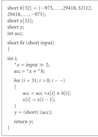
shorth[32]= {−973,. . ., 29418, 32112, 29418,. . .,−973};
shortx[32]; shorty; int acc;
short fir (short input)
{
inti;
∗x=input;
acc=∗x∗∗h2;
for (i=31;i >0;i− −)
{
acc=acc +x[i]∗h[i]2; x[i]=x[i−1];
}
y=(short) (acc);
returny;
}
Algorithm2: Fixed-point C code for the FIR filter before the scal-ing operation optimisation.
the scaling operation cost computation, the transfer of some scaling operations, and the scheduling. The scaling opera-tions are processed by cost-decreasing order. They are moved as long as their cost is equal to one and the accuracy con-straint is fulfilled.
4. EXPERIMENTS AND RESULTS
4.1. Floating-to-fixed-point conversion for a WCDMA receiver
The aim of this part is to show the interest of our approach to obtain an optimised fixed-point specification in the case of a real-life application corresponding to a WCDMA receiver. Especially, this experiment underlines the benefits provided by the data type selection stage to reduce the code execution time.
4.1.1. WCDMA receiver description
The considered application corresponds to a receiver used in the base station for the third-generation telecommunication systems. UMTS (Universal Mobile Telecommunications Sys-tem) is based on the wideband code-division multiple-access (WCDMA) norm [40]. The information data (DPDCH) and the control data (DPCCH) are spread with an orthogonal variable-spreading-factor code (OVSF), and then scrambled by a specific spreading sequence (Kasami codes).
In the receiver part, the complex received signal is made up of different delayed copies of the transmitted signal due to the multipaths inside the radio channel. The RAKE-receiver concept is based on the combination of the different multi-path components to improve the quality of the decision on symbols. Each multipath signal is processed by a finger which
shorth[32]= {−973,. . ., 29418, 32112, 29418,. . .,−973};
shortx[32]; shorty; int acc;
short fir (short input)
{
inti;
∗x=input2;
acc=∗x∗∗h;
for (i=31;i >0;i− −)
{
acc=acc +x[i]∗h[i]; x[i]=x[i−1];
}
y=(short) (acc);
returny;
}
Algorithm3: Fixed-point C code for the FIR filter after the scaling operation optimisation.
correlates the received signal by a spreading code. The RAKE receiver and the different finger structures are detailed in
Figure 14. The signal y(k) corresponds to the combination of the different finger outputsyl(k). To combine the different finger results, the complex amplitudeαlof thelth path must be estimated and removed for each multipath. The symbols are decoded by multiplying the received signal with a syn-chronised version of the code generated in the receiver. The synchronisation between the code and the received signal is realised by a delay-locked loop (DLL).
For each finger, the symbols (DPDCH/DPCCH) are es-timated with the symbol decoder structure presented in
Figure 15. Thanks to the complex multiplication (CM 1) of the received signal by the conjugate of the Kasami code c∗K(n) the unscrambling operation is performed. Then, the phase distortion resulting from the transmission channel is removed with the complex multiplication (CM 2) with the conjugate of the complex amplitude estimation (α∗l). At last, the despreading operation with OVSF code (cOVSFI(n) and cOVSFQ(n)) transforms the wideband received signal into a narrowband signal. This operation decodes the transmitted symbolsyl(k).
4.1.2. Data type selection
Se(n)
Finger 0 Finger 1 Finger 2
y0(k)
y1(k)
y2(k)
A2
+
y(k) yb(k)
xl(n)
z−4 4 DLL early Finger
Un-scramble removingPhase
Symbol decoding DPDCH/DPCCH
decoding
DPDCH
DPCCH
yl
α∗l Channel
estimation
z−2 4 DLL on time DLL
z0 4 DLL late
Figure14: Schematic of the RAKE receiver and the finger for a base station. The RAKE receiver achieves the combination of the different finger results.
× ×
×
×
Se(n)
CM1 CM2
cK∗(n) α∗i
cOVSFI(n)
C3
cOVSFQ(n)
SF
A1
256
SF
256 1 SF
1 256
yl(k)
Figure15: Symbol decoding subsystem for a base-station receiver.
inTable 2 and the word-lengths of the operation operands are reported. These different results have been obtained by using our methodology with different accuracy constraints (SQNRmin). The execution time (Tnorm(
− →
b)) is normalised in relation to the execution time of a classical implementa-tion based on single-precision instrucimplementa-tions (multiplicaimplementa-tion: 16×16⇒32 bits; addition: 32 + 32⇒32 bits).
Before determining the RAKE-receiver fixed-point spec-ification, the accuracy constraint must be defined. This min-imal value of the SQNR (SQNRmin) is defined according to the system performance constraints. In the case of the WCDMA receiver, the performances are specified through the maximal value of the bit error rate (BER). The accu-racy constraint has been defined so that the system out-put BER is slightly modified after the fixed-point conver-sion process. Compared to the floating-point implementa-tion, the maximal BER degradation due to fixed-point com-putation is fixed to 5%. The SQNR minimal value is ob-tained with a floating-point simulation with the technique explained in Section 3.1.3. For the WCDMA receiver, this
accuracy constraint determination process leads to a mini-mal SQNR equal to 12.5 dB.
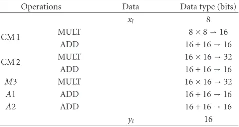
The WCDMA receiver fixed-point specification has been obtained with our methodology. The input data (receiving Nyquist filter output) word-length was fixed to 8 bits. The word-lengths of the main data for the symbol decoding sub-system of the RAKE receiver are summarised inTable 3. For this experiment, the Texas Instruments code generation tool is used to benefit from the high performance of the C com-piler and more particularly the software pipelining tech-nique. Thus, the C source code is modified to include the dif-ferent data types from the fixed-point specification. Intrinsic functions are used to express the data parallelism. The data parallelisation must be achieved by the user to exploit the processor SWP capabilities.
Table2: Results of the complex correlator implementation for dif-ferent data types.Tnormis the execution time normalised in relation
to the classical implementation (impl. 2) execution time.
Si Tnorm SQNR(dB)
Operand word-length (bits) Multiplication Addition bits×bits⇒bits bits + bits⇒bits
1 0.6 51 8×8⇒16 16 + 16⇒16
2 1 89 16×16⇒32 32 + 32⇒32
3 1.55 151 32×16⇒32 32 + 32⇒32 4 2.1 170 32×16⇒64 64 + 64⇒64
Table3: Data word-length for the symbol decoding subsystem of the RAKE receiver. The data and the operations are presented in
Figure 15.
Operations Data Data type (bits)
xl 8
CM 1 MULT 8×8→16
ADD 16 + 16→16
CM 2 MULT 16×16→32
ADD 16 + 16→16
M3 MULT 16×16→32
A1 ADD 16 + 16→16
A2 ADD 16 + 16→16
yl 16
not optimised and thus only the single-precision instruc-tions are used (multiplication: 16×16 ⇒32 bits; addition: 32 + 32⇒32 bits). Given that the two floating-to-fixed-point conversion methods presented inSection 2.1do not optimise the data type, the results obtained with these approaches cor-respond to the classical implementation. In our approach, the code is obtained from the fixed-point specification deter-mined with our floating-to-fixed point conversion method-ology. The accuracy constraint and the DSP architecture of-fer the opportunity to use the SWP instructions. To com-pare these two approaches, the ratioF between the two ex-ecution timesTunopt(−→b) andTopt(−→b) is computed. This im-provement factorF, defined in (15), corresponds to the ac-celeration factor due to the data type selection:
F=Tunopt( − →
b)
Topt(−→b) . (15)
Different experiments have been achieved on the symbol decoding and the synchronisation subsystems for several val-ues of the fingers number. The results, presented inTable 4, underline the benefit of the SWP instructions. Our approach reduces the code execution time by a factor between 1.91 and 3.51.
4.2. Optimisation of the scaling operation location
In this section, some experiments have been conducted to show our approach’s interest to optimise the scaling
Table4: SWP improvement factorF. This factorFcorresponds to the acceleration factor due to the data type selection.
Code execution time
Number improvement factorF
of fingers Symbol decoding Synchronisation
subsystem subsystem
1 2.83 1.91
2 2.79 2.79
4 3.51 3.18
operation location for DSP based on conventional architec-ture. These experiments are achieved with the C50 and the C54x DSPs from Texas Instruments. These two processors are based on a classical MAC structure. The C54x DSP is made up of an accumulator with eight guard bits and a barrel shifter connected to the accumulator register. The C50 offers no guard bits and the scaling capabilities based on specialised shift registers are limited. Aprescalerregister is available to shift the data which are loaded from memory and apostscaler register provides the capability to shift the data when they are stored in memory.
The different experiment results are given inTable 5. The scaling operation execution timeTSOis given before and after the optimisation of the scaling operation location to analyse the improvement due to the optimisation process. The exe-cution timeTSO(number of cycles) corresponds to the appli-cation execution time difference with and without the scaling operations. The accuracy degradationΔSQNR(dB) due to the scaling operation transfers is measured.
The two first applications correspond to a finite impulse response and an infinite impulse response filters. The com-plex correlator achieves the correlation between a comcom-plex signal and a complex bipolar code made up ofNpoints. The four last applications are used in the WCDMA receiver for third-generation telecommunication systems. These applica-tions are described in the previous section. The receivers for the mobile terminal (MT) and for the base station (BS) are similar except for the location of the phase removing process-ing. In the base station the phase removing is achieved during the symbol decoding and in the mobile station the phase re-moving is achieved after the symbol decoding and before the output finger combination.
For the C54x, the guard bits ensure a fixed-point speci-fication with a limited number of scaling operations. Except for the IIR filter, these scaling operations correspond to left shifts required to align the guard bits before storing in mem-ory the data which was in the accumulator register. Thus, these scaling operations cannot be moved and the scaling op-eration optimisation does not reduce the scaling opop-eration cost. In the IIR filter, the guard bits are not sufficient to limit the number of scaling operations. A scaling operation is re-quired to adapt the format of the recursive and the nonre-cursive part outputs. This scaling operation can be moved to reduce the scaling operation cost.