Efficient Hierarchical Entity Classifier Using Conditional Random Fields
Koen Deschacht
Interdisciplinary Centre for Law & IT Katholieke Universiteit Leuven Tiensestraat 41, 3000 Leuven, Belgium
Marie-Francine Moens Interdisciplinary Centre for Law & IT
Katholieke Universiteit Leuven Tiensestraat 41, 3000 Leuven, Belgium
Abstract
In this paper we develop an automatic classifier for a very large set of labels, the WordNet synsets. We employ Conditional Random Fields (CRFs) because of their flexibility to include a wide variety of non-independent features. Training CRFs on a big number of labels proved a problem be-cause of the large training cost. By tak-ing into account the hypernym/hyponym relation between synsets in WordNet, we reduced the complexity of training from O(T M2N G) toO(T(logM)2N G) with only a limited loss in accuracy.
1 Introduction
The work described in this paper was carried out during the CLASS project1. The central objec-tive of this project is to develop advanced learning methods that allow images, video and associated text to be analyzed and structured automatically. One of the goals of the project is the alignment of visual and textual information. We will, for exam-ple, learn the correspondence between faces in an image and persons described in surrounding text. The role of the authors in the CLASS project is mainly on information extraction from text.
In the first phase of the project we build a clas-sifier for automatic identification and categoriza-tion of entities in texts which we report here. This classifier extracts entities from text, and assigns a label to these entities chosen from an inventory of possible labels. This task is closely related to both named entity recognition (NER), which tra-ditionally assigns nouns to a small number of cate-gories and word sense disambiguation (Agirre and
1http://class.inrialpes.fr/
Rigau, 1996; Yarowsky, 1995), where the sense for a word is chosen from a much larger inventory of word senses.
We will employ a probabilistic model that’s been used successfully in NER (Conditional Ran-dom Fields) and use this with an extensive inven-tory of word senses (the WordNet lexical database) to perform entity detection.
In section 2 we describe WordNet and it’s use for entity categorization. Section 3 gives an overview of Conditional Random Fields and sec-tion 4 explains how the parameters of this model are estimated during training. We will drastically reduce the computational complexity of training in section 5. Section 6 describes the implementation of this method, section 7 the obtained results and finally section 8 future work.
2 WordNet
WordNet (Fellbaum et al., 1998) is a lexical database whose design is inspired by psycholin-guistic theories of human lexical memory. English nouns, verbs, adjectives and adverbs are organized in synsets. A synset is a collection of words that have a close meaning and that represent an under-lying concept. An example of such a synset is “person, individual, someone, somebody, mortal, soul”. All these words refer to a human being.
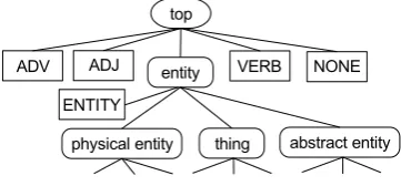
WordNet (v2.1) contains 155.327 words, which are organized in 117.597 synsets. WordNet de-fines a number of relations between synsets. For nouns the most important relation is the hyper-nym/hyponym relation. A noun X is a hypernym of a noun Y if Y is a subtype or instance of X. For example, “bird” is a hypernym of “penguin” (and “penguin” is a hyponym of “bird”). This relation organizes the synsets in a hierarchical tree (Hayes, 1999), of which a fragment is pictured in fig. 1.
Figure 1: Fragment of the hypernym/hyponym tree
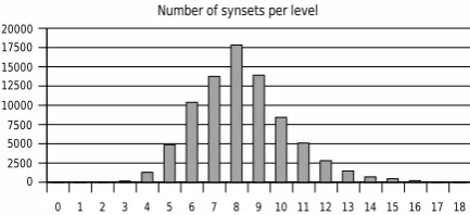
This tree has a depth of 18 levels and maximum width of 17837 synsets (fig. 2).
We will build a classifier using CRFs that tags noun phrases in a text with their WordNet synset. This will enable us to recognize entities, and to classify the entities in certain groups. Moreover, it allows learning the context pattern of a certain meaning of a word. Take for example the sentence “The ambulance took the remains of the bomber to the morgue.” Having every noun phrase tagged with it’s WordNet synset reveals that in this sen-tence, “bomber” is “a person who plants bombs” (and not “a military aircraft that drops bombs dur-ing flight”). Usdur-ing the hypernym/hyponym rela-tions from WordNet, we can also easily find out that “ambulance” is a kind of “car”, which in turn is a kind of “conveyance, transport” which in turn is a “physical object”.
3 Conditional Random Fields
Conditional random fields (CRFs) (Lafferty et al., 2001; Jordan, 1999; Wallach, 2004) is a statistical method based on undirected graphical models. Let Xbe a random variable over data sequences to be labeled andY a random variable over correspond-ing label sequences. All components Yi ofY are
assumed to range over a finite label alphabet K. In this paper X will range over the sentences of a text, tagged with POS-labels andY ranges over the synsets to be recognized in these sentences.
We define G = (V, E) to be an undirected graph such that there is a nodev∈V correspond-ing to each of the random variables representcorrespond-ing an elementYvofY. If each random variableYvobeys
the Markov property with respect to G (e.g., in a first order model the transition probability depends only on the neighboring state), then the model
(Y, X)is a Conditional Random Field. Although the structure of the graph G may be arbitrary, we limit the discussion here to graph structures in
Figure 2: Number of synsets per level in WordNet
which the nodes corresponding to elements of Y form a simple first-order Markov chain.
A CRF defines a conditional probability distri-butionp(Y|X)of label sequences given input quences. We assume that the random variable se-quences X and Y have the same length and use x= (x1, ..., xT)andy= (y1, ..., yT)for an input
sequence and label sequence respectively. Instead of defining a joint distribution over both label and observation sequences, the model defines a condi-tional probability over labeled sequences. A novel observation sequence xis labeled with y, so that the conditional probability p(y|x) is maximized. We define a set of K binary-valued features or feature functionsfk(yt−1, yt,x)that each express some characteristic of the empirical distribution of the training data that should also hold in the model distribution. An example of such a feature is
fk(yt−1, yt,x) =
1 ifxhas POS ‘NN’ and
ytis concept ‘entity’
0 otherwise
(1) Feature functions can depend on the previous (yt−1) and the current (yt) state. Considering K
feature functions, the conditional probability dis-tribution defined by the CRF is
p(y|x) = 1 Z(x)
exp ( T
X
t=1
K
X
k=1
λkfk(yt−1, yt,x) )
(2) where λj is a parameter to model the observed
statistics andZ(x)is a normalizing constant com-puted as
Z(x) = X
y∈Y
exp ( T
X
t=1
K
X
k=1
λkfk(yt−1, yt,x) )
[image:2.595.311.528.55.154.2]It brings together the best of discriminative mod-els and generative modmod-els: (1) It can accommo-date many statistically correlated features of the inputs, contrasting with generative models, which often require conditional independent assumptions in order to make the computations tractable and (2) it has the possibility of context-dependent learning by trading off decisions at different sequence posi-tions to obtain a global optimal labeling. Because CRFs adhere to the maximum entropy principle, they offer a valid solution when learning from in-complete information. Given that in information extraction tasks, we often lack an annotated train-ing set that covers all possible extraction patterns, this is a valuable asset.
Lafferty et al. (Lafferty et al., 2001) have shown that CRFs outperform both MEMM and HMM on synthetic data and on a part-of-speech tagging task. Furthermore, CRFs have been used success-fully in information extraction (Peng and McCal-lum, 2004), named entity recognition (Li and Mc-Callum, 2003; McCallum and Li, 2003) and sen-tence parsing (Sha and Pereira, 2003).
4 Parameter estimation
In this section we’ll explain to some detail how to derive the parameters θ = {λk}, given the
train-ing data. The problem can be considered as a con-strained optimization problem, where we have to find a set of parameters which maximizes the log likelihood of the conditional distribution (McCal-lum, 2003). We are confronted with the problem of efficiently calculating the expectation of each feature function with respect to the CRF model distribution for every observation sequence x in the training data. Formally, we are given a set
of training examples D = nx(i),y(i) oN
i=1 where
each x(i) = n
x1(i), x2(i), ..., x(Ti)o is a sequence
of inputs and y(i) = n
y1(i), y2(i), ..., y(Ti)o is a se-quence of the desired labels. We will estimate the parameters by penalized maximum likelihood, op-timizing the function:
l(θ) =
N
X
i=1
log p(y(i)|x(i)) (3)
After substituting the CRF model (2) in the
like-lihood (3), we get the following expression:
l(θ) = PN
i=1
T
P
t=1
K
P
k=1
λkfk(y(t−i)1, y
(i)
t ,x(i))
−PN
i=1
log Z(x(i))
The functionl(θ)cannot be maximized in closed form, so numerical optimization is used. The par-tial derivates are:
∂l(θ)
∂λk =
N
P
i=1
T
P
t=1
fk(yt(i), y
(i)
t−1,x
(i))
−PN
i=1
T
P
t=1
P
y,y′
fk(y′, y,x(i))p(y′, y|x(i))
(4) Using these derivates, we can iteratively adjust the parameters θ (with Limited-Memory BFGS (Byrd et al., 1994)) untill(θ)has reached an opti-mum. During each iteration we have to calculate p(y′, y|x(i)). This can be done, as for the
Hid-den Markov Model, using the forward-backward algorithm (Baum and Petrie, 1966; Forney, 1996). This algorithm has a computational complexity of O(T M2) (whereT is the length of the sequence andM the number of the labels). We have to exe-cute the forward-backward algorithm once for ev-ery training instance during evev-ery iteration. The total cost of training a linear-chained CRFs is thus:
O(T M2N G)
whereNis the number of training examples andG the number of iterations. We’ve experienced that this complexity is an important delimiting factor when learning a big collection of labels. Employ-ing CRFs to learn the 95076 WordNet synsets with 20133 training examples was not feasible on cur-rent hardware. In the next section we’ll describe the method we’ve implemented to drastically re-duce this complexity.
5 Reducing complexity
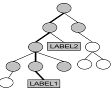
Figure 3: Fragment of the tree used for labeling
5.1 Hierarchical feature selection
To reduce the complexity of CRFs, we assign a selection of features to every node in the hierar-chical tree. As discussed in section 2 WordNet de-fines a relation between synsets which organises the synsets in a tree. In its current form this tree does not meet our needs: we need a tree where every label used for labeling corresponds to ex-actly one leaf-node, and no label corresponds to a non-leaf node. We therefor modify the existing tree. We create a new top node (“top”) and add the original tree as defined by WordNet as a subtree to this top-node. We add leaf-nodes corresponding to the labels “NONE”, “ADJ”, “ADV”, “VERB” to the top-node and for the other labels (the noun synsets) we add a leaf-node to the node represent-ing the correspondrepresent-ing synset. For example, we add a node corresponding to the label “ENTITY” to the node “entity”. Fig. 3 pictures a fraction of this tree. Nodes corresponding to a label have an uppercase name, nodes not corresponding to a la-bel have a lowercase name.
We use vto denote nodes of the tree. We call the top conceptvtopand the conceptv+the parent of v, which is the parent of v−. We callA
v the
collection of ancestors of a conceptv, includingv itself.
We will now show how we transform a regular CRF in a CRF that uses hierarchical feature selec-tion. We first notice that we can rewrite eq. 2 as
p(y|x) = 1 Z(x)
T
Y
t=1
G(yt−1, yt,x)
withG(yt−1, yt,x) =exp(
K
P
k=1
λkfk(yt−1, yt,x))
We rewrite this equation because it will enable us to reduce the complexity of CRFs and it has the property that p(yt|yt−1,x) ≈ G(yt−1, yt,x) which we will use in section 5.3.
We now define a collection of features Fv for
every nodev. Ifvis leaf-node, we defineFvas the
collection of featuresfk(yt−1, yt,x)for which it is possible to find a nodevt−1and inputxfor which fk(vt−1, v,x) 6= 0. Ifvis a non-leaf node, we de-fineFvas the collection of featuresfk(yt−1, yt,x) (1) which are elements ofFv−for every child node
v−ofv and (2) for everyv−
1 and v
−
2, children of
v,it is valid that for every previous labelvt−1and
inputx fk(vt−1, v−1,x) =fk(vt−1, v2−,x).
Informally, Fv is the collection of features
which are useful to evaluate for a certain node. For the leaf-nodes, this is the collection of features that can possibly return a non-zero value. For non-leaf nodes, it’s useful to evaluate features belonging to Fv when they have the same value for all the
de-scendants of that node (which we can put to good use, see further).
We defineF′
v =Fv\Fv+ wherev+is the parent
of labelv. For the top nodevtopwe defineF′
vtop =
Fvtop. We also set
G′
(yt−1, yt,x) =exp
X
fk∈F′ yt
λkfk(yt−1, yt,x)
We’ve now organised the collection of features in such a way that we can use the hierarchical rela-tions defined by WordNet when determining the probability of a certain labeling y. We first see that
G(yt−1, yt,x) = exp
X
fk∈Fyt
λkfk(yt−1, yt,x)
= G(yt−1, y+t , x)G
′
(yt−1, yt, x)
= ...
= Y
v∈Ayt
G′
(yt−1, v, x)
we can now determine the probability of a labeling
y, given inputx
p(y|x) = 1 Z(x)
T
Y
t=1
Y
v∈Ayt
G′
(yt−1, v,x) (5)
5.2 Labeling
The standard method to label a sentence with CRFs is by using the Viterbi algorithm (Forney, 1973; Viterbi, 1967) which has a computational complexity ofO(T M2). The basic idea to reduce this computational complexity is to select the best labeling in a number of iterations. In the first itera-tion, we label every word in a sentence with a label chosen from the top-level labels. After choosing the best labeling, we refine our choice (choose a child label of the previous chosen label) in subse-quent iterations until we arrive at a synset which has no children. In every iteration we only have to choose from a very small number of labels, thus breaking down the problem of selecting the correct label from a large number of labels in a number of smaller problems.
Formally, when labeling a sentence we find the label sequence y such that y has the maximum probability of all labelings. We will estimate the best labeling in an iterative way: we start with the best labeling ytop−1 = {y1top−1, ..., ytopT −1} choosing only from the children yttop−1of the top node. The probability of this labelingytop−1is
p(ytop−1|x) = 1 Z′(
x)
T
Y
t=1
G′
(yt−1, ytop
−1
t ,x)
where Z′
(x) is an appropriate normalizing con-stant. We now select a labelingytop−2 so that on every position tnodeyttop−2 is a child of ytopt −1. The probabilty of this labeling is (following eq. 5)
p(ytop−2|x) = 1 Z′(
x)
T
Y
t=1
Y
v∈A
ytop−2 t
G′
(yt−1, v,x)
After selecting a labeling ytop−2 with maximum probability, we proceed by selecting a labeling ytop−3 with maximum probability etc.. We pro-ceed using this method until we reach a labeling in which everyytis a node which has no children
and return this labeling as the final labeling. The assumption we make here is that if a node vis selected at positiontof the most probable la-belingytop−s the childrenv−have a larger prob-ability of being selected at position tin the most probable labelingytop−s−1. We reduce the num-ber of labels we take into consideration by stating that for every conceptvfor whichv 6=yttop−s, we set G′
(yt−1, v −
t ,x) = 0 for every child v
−
[image:5.595.361.473.51.140.2]ofv. This reduces the space of possible labelings dras-tically, reducing the computational complexity of
Figure 4: Nodes that need to be taken into account during the forward-backward algorithm
the Viterbi algorithm. If q is the average number of children of a concept, the depth of the tree is logq(M). On every level we have to execute the
Viterbi algorithm for q labels, thus resulting in a total complexity of
O(T logq(M)q2) (6)
5.3 Training
We will now discuss how we reduce the compu-tational complexity of training. As explained in section 4 we have to estimate the parameters λk
that optimize the functionl(θ). We will show here how we can reduce the computational complex-ity of the calculation of the partial derivates ∂l∂λ(θ)
k
(eq. 4). The predominant factor with regard to the computational complexity in the evaluation of this equation is the calculation of p(yt−1, y|x(i)).
Recall we do this with the forward-backward al-gorithm, which has a computational complexity ofO(T M2). We reduce the number of labels to improve performance. We will do this by mak-ing the same assumption as in the previous sec-tion: for every concept v at level s, for which v 6= ytopt −s, we set G′
(yt−1, vt−,x) = 0 for
every child v− of v. Since (as noted in sect.
5.2) p(vt|yt−1,x) ≈ G(yt−1, vt,x), this has the consequence that p(vt|yt−1,x) = 0 and that p(vt, yt−1|x) = 0. Fig. 4 gives a graphical repre-sentation of this reduction of the search space. The correct label here is “LABEL1” , the grey nodes have a non-zerop(vt, yt−1|x)and the white nodes have a zerop(vt, yt−1|x).
In the forward backward algorithm we only have to account every node v that has a non-zero p(v, yt−1|x). As can be easily seen from fig. 4,
the number of nodes is qlogqM, where q is the
average number of children of a concept. The to-tal complexity of running the forward-backward algorithm is O(T(q logqM)2). Since we have to
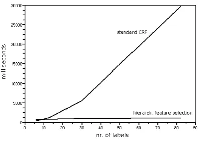
compu-Figure 5: Time needed for one training cycle
tation for every training instance we find the total training cost
O(T(q logqM)2N G) (7)
6 Implementation
To implement the described method we need two components: an interface to the WordNet database and an implementation of CRFs using a hierar-chical model. JWordNet is a Java interface to WordNet developed by Oliver Steele (which can be found on http://jwn.sourceforge. net/). We used this interface to extract the Word-Net hierarchy.
An implementation of CRFs using the hierar-chical model was obtained by adapting the Mallet2 package. The Mallet package (McCallum, 2002) is an integrated collection of Java code useful for statistical natural language processing, document classification, clustering, and information extrac-tion. It also offers an efficient implementation of CRFs. We’ve adapted this implementation so it creates hierarchical selections of features which are then used for training and labeling.
We used the Semcor corpus (Fellbaum et al., 1998; Landes et al., 1998) for training. This cor-pus, which was created by the Princeton Univer-sity, is a subset of the English Brown corpus con-taining almost 700,000 words. Every sentence in the corpus is noun phrase chunked. The chunks are tagged by POS and both noun and verb phrases are tagged with their WordNet sense. Since we do not want to learn a classification for verb synsets, we replace the tags of the verbs with one tag “VERB”.
[image:6.595.74.276.68.208.2]2http://mallet.cs.umass.edu/
Figure 6: Time needed for labeling
7 Results
The major goal of this paper was to build a clas-sifier that could learn all the WordNet synsets in a reasonable amount of time. We will first discuss the improvement in time needed for training and labeling and then discuss accuracy.
We want to test the influence of the number of labels on the time needed for training. Therefor, we created different training sets, all of which had the same input (246 sentences tagged with POS la-bels), but a different number of labels. The first training set only had 5 labels (“ADJ”, “ADV”, “VERB”, “entity” and “NONE”). The second had the same labels except we replaced the label “en-tity” with either “physical en“en-tity”, “abstract en“en-tity” or “thing”. We continued this procedure, replac-ing parent nouns labels with their children (i.e. hyponyms) for subsequent training sets. We then trained both a CRF using a hierarchical feature se-lection and a standard CRF on these training sets.
Fig. 5 shows the time needed for one iteration of training with different numbers of labels. We can see how the time needed for training slowly increases for the CRF using hierarchical feature selection but increases fast when using a standard CRF. This is conform to eq. 7.
Fig. 6 shows the average time needed for la-beling a sentence. Here again the time increases slowly for a CRF using hierarchical feature selec-tion, but increases fast for a standard CRF, con-form to eq. 6.
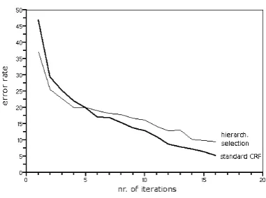
[image:6.595.311.508.69.210.2]can differ considerable from the error rate on un-seen data.
After these tests on a small section of the Sem-cor Sem-corpus, we trained a CRF using hierarchi-cal feature selection on 7/8 of the full corpus. We trained for 23 iterations, which took approx-imately 102 hours. Testing the model on the re-maining 1/8 of the corpus resulted in an accuracy of 77.82%. As reported in (McCarthy et al., 2004), a baseline approach that ignors context but simply assigns the most likely sense to a given word ob-tains a accuracy of 67%. We did not have the pos-sibility to compare the accuracy of this model with a standard CRF, since as already stated, training such a CRF takes impractically long, but we can compare our systems with existing WSD-systems. Mihalcea and Moldovan (Mihalcea and Moldovan, 1999) use the semantic density between words to determine the word sense. They achieve an ac-curacy of 86.5% (testing on the first two tagged files of the Semcor corpus). Wilks and Stevenson (Wilks and Stevenson, 1998) use a combination of knowledge sources and achieve an accuracy of 92%3. Note that both these methods use additional knowledge apart from the WordNet hierarchy.
The sentences in the training and testing sets were already (perfectly) POS-tagged and noun chunked, and that in a real-life situation addi-tional preprocessing by a POS-tagger (such as the LT-POS-tagger4) and noun chunker (such as de-scribed in (Ramshaw and Marcus, 1995)) which will introduce additional errors.
8 Future work
In this section we’ll discuss some of the work we plan to do in the future. First of all we wish to evaluate our algorithm on standard test sets, such as the data of the Senseval conference5, which tests performance on word sense disambiguation, and the data of the CoNLL 2003 shared task6, on named entity recognition.
An important weakness of our algorithm is the fact that, to label a sentence, we have to traverse the hierarchy tree and choose the correct synsets at every level. An error at a certain level can not be recovered. Therefor, we would like to perform
3
This method was tested on the Semcore corpus, but use the word senses of the Longman Dictionary of Contemporary English
4
http://www.ltg.ed.ac.uk/software/ 5http://www.senseval.org/
[image:7.595.317.508.67.209.2]6http://www.cnts.ua.ac.be/conll2003/
Figure 7: Error rate during training
some a of beam-search (Bisiani, 1992), keeping a number of best labelings at every level. We strongly suspect this will have a positive impact on the accuracy of our algorithm.
As already mentioned, this work is carried out during the CLASS project. In the second phase of this project we will discover classes and at-tributes of entities in texts. To accomplish this we will not only need to label nouns with their synset, but we also need to label verbs, adjec-tives and adverbs. This can become problem-atic as WordNet has no hypernym/hyponym rela-tion (or equivalent) for the synsets of adjectives and adverbs. WordNet has an equivalent relation for verbs (hypernym/troponym), but this structures the verb synsets in a big number of loosely struc-tured trees, which is less suitable for the described method. VerbNet (Kipper et al., 2000) seems a more promising resource to use when classify-ing verbs, and we will also investigate the use of other lexical databases, such as ThoughtTrea-sure (Mueller, 1998), Cyc (Lenat, 1995), Open-mind Commonsense (Stork, 1999) and FrameNet (Baker et al., 1998).
Acknowledgments
The work reported in this paper was supported by the EU-IST project CLASS (Cognitive-Level Annotation using Latent Statistical Structure, IST-027978).
References
Computational Linguistics (Coling’96), pages 16– 22, Copenhagen, Denmark.
C. F. Baker, C. J. Fillmore, and J. B. Lowe. 1998. The Berkeley Framenet project. In Proceedings of the COLING-ACL.
L. E. Baum and T. Petrie. 1966. Statistical in-ference for probabilistic functions of finite state markov chains. Annals of Mathematical Statistics,, 37:1554–1563.
R. Bisiani. 1992. Beam search. In S. C. Shapiro, editor, Encyclopedia of Artificial Intelligence, New York. Wiley-Interscience.
Richard H. Byrd, Jorge Nocedal, and Robert B. Schn-abel. 1994. Representations of quasi-newton matri-ces and their use in limited memory methods. Math. Program., 63(2):129–156.
C. Fellbaum, J. Grabowski, and S. Landes. 1998. Per-formance and confidence in a semantic annotation task. In C. Fellbaum, editor, WordNet: An Elec-tronic Lexical Database. The MIT Press.
G. D. Forney. 1973. The viterbi algorithm. In Pro-ceeding of the IEEE, pages 268 – 278.
G. D. Forney. 1996. The forward-backward algo-rithm. In Proceedings of the 34th Allerton Confer-ence on Communications, Control and Computing, pages 432–446.
Brian Hayes. 1999. The web of words. American Scientist, 87(2):108–112, March-April.
Michael I. Jordan, editor. 1999. Learning in Graphical Models. The MIT Press, Cambridge.
K. Kipper, H.T. Dang, and M. Palmer. 2000. Class-based construction of a verb lexicon. Proceedings of the Seventh National Conference on Artificial In-telligence (AAAI-2000).
J. Lafferty, A. McCallum, and F. Pereira. 2001. Con-ditional random fields: Probabilistic models for seg-menting and labeling sequence data. In Proceed-ings of the 18th International Conference on Ma-chine Learning.
S. Landes, C. Leacock, and R.I. Tengi. 1998. Build-ing semantic concordances. In C. Fellbaum, editor, WordNet: An Electronic Lexical Database. The MIT Press.
D. B. Lenat. 1995. Cyc: A large-scale investment in knowledge infrastructure. Communications of the ACM, 38(11):32–38.
Wei Li and Andrew McCallum. 2003. Rapid develop-ment of hindi named entity recognition using con-ditional random fields and feature induction. ACM Transactions on Asian Language Information Pro-cessing (TALIP), 2(3):290–294.
Andrew McCallum and Wei Li. 2003. Early results for named entity recognition with conditional ran-dom fields, feature induction and web-enhanced lex-icons. In Walter Daelemans and Miles Osborne, ed-itors, Proceedings of CoNLL-2003, pages 188–191. Edmonton, Canada.
Andrew Kachites McCallum. 2002. Mal-let: A machine learning for language toolkit. http://mallet.cs.umass.edu.
A. McCallum. 2003. Efficiently inducing features of conditional random fields. In Proceedings of the Nineteenth Conference on Uncertainty in Artificial Intelligence.
D. McCarthy, R. Koeling, J. Weeds, and J. Carroll. 2004. Using automatically acquired predominant senses for word sense disambiguation. In Proceed-ings of the ACL SENSEVAL-3 workshop, pages 151– 154, Barcelona, Spain.
R. Mihalcea and D.I. Moldovan. 1999. A method for word sense disambiguation of unrestricted text. In Proceedings of the 37th conference on Associa-tion for ComputaAssocia-tional Linguistics, pages 152–158. Association for Computational Linguistics Morris-town, NJ, USA.
Erik T. Mueller. 1998. Natural language processing with ThoughtTreasure. Signiform, New York.
F. Peng and A. McCallum. 2004. Accurate infor-mation extraction from research papers using con-ditional random fields. In Proceedings of Human Language Technology Conference and North Amer-ican Chapter of the Association for Computational Linguistics (HLT-NAACL), pages 329–336.
L.A. Ramshaw and M.P. Marcus. 1995. Text chunking using transformation-based learning. In Proceed-ings of the Third ACL Workshop on Very Large Cor-pora, pages 82–94. Cambridge MA, USA.
F. Sha and F. Pereira. 2003. Shallow parsing with con-ditional random fields. In Proceedings of Human Language Technology, HLT-NAACL.
D. Stork. 1999. The openmind initiative. IEEE Intelli-gent Systems & their applications, 14(3):19–20.
A. J. Viterbi. 1967. Error bounds for convolutional codes and an asymptotically optimal decoding algo-rithm. IEEE Trans. Informat. Theory, 13:260–269.
Hanna M. Wallach. 2004. Conditional random fields: An introduction. Technical Report MS-CIS-04-21., University of Pennsylvania CIS.
Y. Wilks and M. Stevenson. 1998. Word sense disam-biguation using optimised combinations of knowl-edge sources. Proceedings of COLING/ACL, 98.