value_at_risk

(1)

estimation of value-at-risk and expected shortfall based on nonlinear models of return dynamics and Extreme Value Theory

by

Carlos Martins-Filho Feng Yao

Department of Economics Department of Economics Oregon State University and Oregon State University

Ballard Hall 303 Ballard Hall 303

Corvallis, OR 97331-3612 USA Corvallis, OR 97331-3612 USA email: [email protected] email: [email protected] Voice: + 1 541 737 1476 Voice: + 1 541 737 2321

Fax: + 1 541 737 5917 Fax: + 1 541 737 5917

December, 2002

Abstract: We propose an estimation procedure forvalue at risk (VaR) andexpected shortfall (TailVaR) for conditional distributions of a time series of returns on a ¯nancial asset. Our approach combines a local polynomial estimator of conditional mean and volatility functions in a conditional heterocedastic autore-gressive nonlinear (CHARN) model with Extreme Value Theory for estimating quantiles of the conditional distribution. We investigate the ¯nite sample properties of our method and contrast them with alternatives, including the method recently proposed by McNeil and Frey(2000), in an extensive Monte Carlo study. The method we propose outperforms the estimators currently available in the literature.

Keywords and Phrases: Risk Measures; Value at Risk; CHARN Models; Extreme Value Theory.

(2)

1 Introduction

The measurement of market risk to which ¯nancial institutions are exposed has become an important in-strument for market regulators, portfolio managers and for internal risk control. As evidence of this growing importance, the Bank of International Settlements (Basel Committee,1996) has imposed capital adequacy requirements on ¯nancial institutions that are based on measurements of market risk. Furthermore, there has been a proliferation of risk measurement tools and methodologies in ¯nancial markets (Risk,1999). Two quantitative and synthetic measures of market risk have emerged in the ¯nancial literature, Value-at-Risk or VaR (RiskMetrics,1995) and Expected Shortfall or TailVaR (Artzner et al.,1999). From a statistical perspective these risk measures have straightforward de¯nitions. Let fYtg be a stochastic process repre-senting returns on a given portfolio, stock, bond or market index, where t indexes a discrete measure of time and Ft denotes either the marginal or the conditional distribution (normally conditioned on the lag historyfYt¡kgM¸k¸1;for some M = 1;2; :::) ofYt. For 0< ® <1, the®-VaR of Ytis simply the®-quantile associated with Ft.1 _{Expected shortfall is de¯ned as} _E

F_ty(Yt) where the expectation is taken with respect to F_ty, the truncated distribution associated withYt > y where y is a speci¯ed threshold level. When the thresholdyis taken to be ®-VaR, then we refer to®-TailVaR.

Accurate estimation of VaR and TailVaR depends crucially on the ability to estimate the tails of the probability density functionft associated withFt. Conceptually, this can be accomplished in two distinct ways: a) direct estimation of ft, or b) indirectly through a suitably de¯ned (parametric) model for the tails of ft. Unless estimation is based on a correct speci¯cation of ft (up to a ¯nite set of parameters), direct estimation will most likely provide a poor ¯t for its tails, since most observed data will likely take values away from the tail region of ft (Diebold et al., 1998). As a result, a series of indirect estimation methods based on Extreme Value Theory (EVT) has recently emerged, including Embrechts et al.(1999), Longin(2000) and McNeil and Frey(2000). These indirect methods are based on approximatingonlythe tails

1_{We will assume throughout this paper that}_F

(3)

offt by an appropriately de¯ned parametric density function.

In the case whereftis a conditional density associated with a stochastic process of returns on a ¯nancial asset, a particularly promising approach is the two stage estimation procedure for conditional VaR and TailVaR suggested by McNeil and Frey. They envision a stochastic process whose evolution can be described as,

Yt=¹t+¾t²tfort= 1;2; :::; (1)

where ¹t is the conditional mean, ¾t is the square root of the conditional variance (volatility) and f²tg

is an independent, identically distributed process with mean zero, variance one and marginal distribution F². Based on a sample fytgnt=1, the ¯rst stage of the estimation produces ^¹t and ^¾t. In the second stage, et = yt¡_^_¾_t¹^t fort = 1; :::; n are used to estimate a generalized pareto density approximation for the tails of ft, which in turn produce VaR and TailVaR sequences for the conditional distribution ofYt. Backtesting of their method (using various ¯nancial return series) against some widely useddirectestimation methods that assume a speci¯c form for the distribution of²t(gaussian, student-t) have produced favorable, albeit speci¯c results. Although encouraging, the backtesting results are speci¯c to the series analyzed and uninformative regarding the statistical properties of the two stage estimators for VaR and TailVaR. Furthermore, since various ¯rst and second stage estimators can be proposed, the important question on how to best implement the two stage procedure remains unexplored.

(4)

can be rather restrictive, speci¯cally with regards to volatility asymmetry, we consider a nonparametric markov chain model (HÄardle and Tsybakov,1997 and Hafner,1998) for_fYtgdynamics, as well as an improved nonparametric estimation procedure for the conditional volatility of the returns (Fan and Yao,1998). The objective is to have in place a ¯rst stage estimator that is general enough to accommodate nonlinearities that have been regularly veri¯ed in empirical work (Andreou et al.,2001, Hafner,1998, Patton,2001 and Tauchen,2001). We also propose an alternative estimator for the EVT inspired parametric tail model in the second stage. The estimation we propose, which derives from L-Moment Theory (Hosking,1987), is easier and faster to implement, and in ¯nite samples outperforms, the constrained maximum likelihood estimation methods that have prevailed in the empirical ¯nance literature.

(5)

2 Stochastic Properties of

_f

Y

t

g

and Estimation

The practical use of discrete time stochastic processes such as (1) to model asset price returns has proceeded by making speci¯c assumptions on¹t,¾tand²t. Generally, it is assumed that up to a ¯nite set of parameters the functional speci¯cations for¹t and¾t are known and that the conditioning set over which these expec-tation are taken depends only on past realizations of the process.2 _{Furthermore, to facilitate estimation,} speci¯c distributional assumptions are normally made on ²t. ARCH, GARCH, EGARCH, IGARCH and many other variants can be grouped according to this general description. Their success in ¯tting observed data, producing accurate forecasts, and the ease with which they can be estimated depends largely on these assumptions. In fact, the great profusion of ARCH type models is the result of an attempt to accommo-date empirical regularities that have been repeatedly observed in ¯nancial return series. More recently, a number of papers have emerged (Carroll, HÄardle and Mammen,2002, HÄardle and Tsybakov,1997, Masry and Tj¿stheim,1995) which provide a less restrictive nonparametric or semiparametric modeling of¹t,¾t, as well as ²t. These models are in general more di±cult to estimate than their parametric counterparts, but there can be substantial inferential gains if the parametric models are misspeci¯ed or unduly restrictive.

Our interest is in obtaining estimates for®-VaR and®-TailVaR associated with the conditional density ft, where in general conditioning is on the ¯ltrationMt¡1=¾(fYs:M < s·t¡1g), where¡1 ·M ·t¡1. We denote such conditional densities byf(YtjMt¡1) fort= 2;3; :::. Lettingq(®) =F²¡1(®) be the quantile ofF²and given thatF²(x) =F(¹t+¾txjMt¡1) we have that®-VaR forf(yjMt¡1) is given by,

F¡1(®jMt¡1) =¹t+¾tq(®): (2)

Similarly,®-TailVaR forf(yjMt_¡1) is given by,

E¡YtjYt> F¡1(®jMt¡1); Mt¡1 ¢

(6)

Hence, the estimation of®-VaR and®-TailVaR can be viewed as a process of estimation for the unknown functionals in (2) and (3). We start by considering the following nonparametric speci¯cations for¹t,¾tand the process Yt. Assume that_f(Yt; Yt_¡1)0g is a two dimensional strictly stationary process with conditional mean functionE(YtjYt¡1 = x) = m(x) and conditional variance E

¡

(Yt¡m(x))2jYt¡1=x ¢

=¾2_(x) _>_0. The process is described by the following markov chain of order 1,

Yt=m(Yt_¡1) +¾(Yt_¡1)²tfort= 1;2; ::: ; (4)

where ²tis an independent strictly stationary process with unknown marginal distributionF² that is abso-lutely continuous with mean zero and unit variance. Note that the conditional skewness,®3(x) and kurtosis, ®4(x) of the conditional density ofYtgiven Yt¡1 =xare given by, ®3(x) =E(²3t) and ®4(x) = E(²4t). We assume that such moments exist and are continuous and that m(x) and ¾2_{(x) have uniformly continuous} second derivatives on an open set containingx.

Recursion (4) is the conditional heterocedastic autoregressive nonlinear (CHARN) model of Diebolt and Guµegan(1993), HÄardle and Tsybakov(1997) and Hafner(1998). It is a special case (one lag) of the nonlinear-ARCH model treated by Masry and Tj¿stheim(1995). The CHARN model provides a generalization for the popular GARCH(1,1) model in thatm(x) is a nonparametric function, and most importantly¾2(x) is not a linear function ofYt2¡1. The symmetry inYt¡1of the conditional variance in GARCH models is a particularly undesirable restriction when modeling ¯nancial time series due to the empirically well documentedleverage e®ect (Chen, 2001, Ding, Engle and Granger,1993, Hafner,1998 and Patton,2001). However, (4) is more restrictive than traditional GARCH models in that its markov property restricts its ability to e®ectively model the longer memory that is commonly observed in return processes.3 _{Estimation of the CHARN model} is relatively simple and provides much of its appeal in our context.

3_{The model of Masry and Tj¿stheim(1995) and equations (2) and (3) in Carrol, HÄ}_{ardle and Mammen(2002) provide a full}

nonparametric generalization of ARCH and GARCH(1,1) models. However, nonparametric estimators for the latter model are unavailable and for the former, convergence of the proposed estimators formand¾2 _{is extremely slow as the number of lags}

(7)

2.1 First Stage Estimation

The estimation ofm(x) and¾2_{(x) in (4) was considered by HÄ}_{ardle and Tsybakov(1997). Unfortunately, their} procedure for estimating the conditional variance ¾2_{(x) su®ers from signi¯cant bias and does not produce} estimators that are constrained to be positive. Furthermore, the estimator is not asymptotically design adaptive to the estimation of m, i.e., the asymptotic properties of their estimator for conditional volatility is sensitive to how well mis estimated. We therefore consider an alternative estimation procedure due to Fan and Yao(1998), which is described as follows. First, we estimate m(x) using the local linear estimator of Fan(1992). Let W(x); K(x) :_{< ! <} be symmetric kernel functions, y in the support of the conditional density ofYtandh(n),h1(n) be sequences of positive real numbers - bandwidths - such thath(n); h1(n)!0 asn! 1. Let

( ^¯;¯1)^ 0 =argmin¯;¯1

n X

t=2

(yt¡¯¡¯1(yt_¡1¡y))2K µ

yt_¡1¡y h(n)

¶ ;

then the local linear estimator ofm(y) is ^m(y) = ^¯(y). Second, let ^rt= (yt¡m(yt^ ¡1))2, and de¯ne,

(^´;´^1)0=argmin´;´1

n X

t=2

(^rt¡´¡´1(yt¡1¡y))2W µ

yt¡1¡y h1(n)

¶ ;

then the local linear estimator of¾2_{(y) is ^}_¾2_{(y) = ^}_´(y).

It is clear that an important element of the nonparametric estimation ofmand¾2_{is the selection of the} sequence of bandwidths h(n) andh1(n). We select the bandwidths using the data driven plug-in method of Ruppert, Sheather and Wand(1995) and denote them by ^h(n) and ^h1(n). ^h(n) and ^h1(n) are obtained based on the following regressand-regressor sequencesf(yt; yt_¡1)gn

(8)

context of the CHARN model the ¯rst stage estimators for¹tand¾_t2in (2) and (3) are respectively ^m(yt_¡1) and ^¾2(yt_¡1).

2.2 Second Stage Estimation

In the second stage of the estimation we obtain estimators forq(®) andE(²tj²t> q(®)). The estimation is based on a fundamental result from extreme value theory. To state it, we need some basic de¯nitions. Let q2 < be such that q < ²F, where ²F =supfx2 < :F²(x)<1g is the right endpoint of F², the marginal distribution of the iid processn²t=Yt¡_¾_t¹t

o

. De¯ne the distribution of the excesses of ²over u, Z =²¡u, for a nonstochasticuas,

¡(x; u) =P(Z·xj² > u);

and the generalized pareto distribution - GPD (with location parameter equal to zero) by,

G(x;¯; Ã) = 1¡ µ

1 +Ãx ¯

¶¡1=Ã ; x2D

whereD= [0;1) ifÃ¸0 andD= [0;¡¯=Ã] ifÃ <0. By a theorem of Pickands(1975) ifF²2H then for some positive function¯(u),

limu!²Fsup0<x<²F¡uj¡(x; u)¡G(x;¯(u); Ã)j= 0: (5)

The class H is the maximum domain of attraction of the generalized extreme value distribution (Lead-better et al., 1983). Equation (5) provides a parametric approximation for the distribution of the excesses of²overuwhose validity and precision depends on whetherF²2H anduis large enough. The question of what distribution functions belong toH has been addressed by Haan(1976) and for our purposes it su±ces to observe that it comprises most of the absolutely continuous distributions used in statistics.5

(9)

First stage estimators ^¹tand ^¾2

t can be used to produce a sequence of standardized residuals n

which can be used to estimate the tails of f² based on (5). For this purpose we order the residuals such thatej:n is thejth largest residual, i.e.,e1:n¸e2:n¸:::¸en:n and obtaink < n excesses overek+1:n given byfej:n¡ek+1:ngkj=1, which will be used for estimation of a GPD. By ¯xingk we in e®ect determine the residuals that are used for tail estimation and randomly select the threshold. It is easy to show that for k=n > ®and estimates ^¯ and ^Ã,q(®) andE(²tj²t> q(®)) can be estimated by,

It is clear that these estimators and their properties depend on the choice ofk. This question has been studied by McNeil and Frey (2000) and is also addressed in the Monte Carlo study in section 4 of this paper. Combining the estimators in (6) and (7) with ¯rst stage estimators, and using (2) and (3) gives estimators for®¡V aRand®¡T ailV aR.

We now discuss the estimation of ¯ and Ã. Given the results in Smith(1984,1987), estimation of the GPD parameters has normally been done by constrained maximum likelihood (ML). Here we propose an alternative estimator. Traditionally, raw moments have been used to describe the location and shape of distribution functions. An alternative approach is based on L-moments (Hosking, 1990). Here, we provide a brief justi¯cation for its use and direct the reader to Hosking's paper for a more thorough understanding. LetF²be a distribution function associated with a random variable²andq(u) : (0;1)! <its quantile. The rth _{L-moment of}_² _{is given by,}

¸r= Z 1

0

(10)

where Pr(u) =Pr_k=0pr;kuk andpr;k = (¡_(k!)1)r2¡_(rk(r+k)!_¡_k)! , which contrasts with raw moments ¹r =

R1 0 q(u)

r_du.

Theorem 1 in Hosking(1990) gives the following justi¯cation for using L-moments: a)¹1 is ¯nite if and only if¸rexist for all r; b) a distributionF²with ¯nite ¹1is uniquely characterized by¸r for all r.

L-moments can be used to estimate a ¯nite number of parametersµ 2 £ that identify a member of a family of distributions. SupposefF²(µ) :µ2£½ <pg,pa natural number, is a family of distributions which is known up toµ. A sample f²tgT

t=1 is available and the objective is to estimateµ. Since, ¸r, r= 1;2;3::: uniquely characterizesF, µmay be expressed as a function of¸r. Hence, if estimators ^¸r are available, we may obtain ^µ(^¸1;¸2; :::). From (8), ^^ ¸r = Pr_k=0pr_¡1;k¯k where ¯k =R₀1q(u)uk_{du. Given the sample, we} de¯ne ²k;T to be the kth smallest element of the sample, such that²1;T ·²2;T ·:::· ²T;T. An unbiased estimator of¯k is

^

¯k =T¡1 T X

j=k+1

(j¡1)(j¡2):::(j¡r) (T¡1)(T¡2):::(T ¡r)²j;T and we de¯ne ^¸r =

Pr

k=0pr¡1;k¯^k. IfF² is a generalized pareto distribution with µ = (¹; ¯; Ã), it can be shown that¹=¸1¡(2+Ã)¸2,¯= (1+Ã)(2+Ã)¸2,Ã= 1¡3(¸3=¸2)

1+(¸3=¸2). In our case, where¹= 0,¯ = (1+Ã)¸1,

Ã=¸1=¸2¡2 we de¯ne the following L-moment estimators forÃ and¯,

^ Ã=¸^1

^ ¸2

¡2 and ^¯ = (1 + ^·)^¸1:

(11)

2.3 Alternative First Stage Estimators

Here we de¯ne three alternatives to the ¯rst stage estimation discussed above. The ¯rst is the quasi maxi-mum likelihood estimation (QMLE) method used by McNeil and Frey. In essence it involves estimating by maximum likelihood the following regression model,

Yt=µ1Yt_¡1+¾t²tfort= 1;2; ::: (9)

where ²t » N IID(0;1) and ¾t2 = °0+°1(Yt¡1¡µ1Yt¡2)2+°2¾2t¡1. We will refer to this procedure as GARCH-N. The second alternative estimator we consider is identical to the ¯rst procedure but assumes that the²t are iid with a standardized Student-t density, denoted byfs(º), whereº >2 is a parameter to be estimated together µ1; °0; °1; °2 by maximum likelihood. This estimator has gained popularity in that theYtinherits the leptokurdicity of²t, a characteristic of ¯nancial asset returns that have been abundantly reported in the literature. We refer to this procedure as GARCH-T.

The third estimator we consider is based on the Student-t autoregressive (StAR(1)) model in Spanos(2002). This model can be viewed as a special case of the CHARN model. f(Yt; Yt¡1)0g is taken to be a strictly

stationary two dimensional vector process with Markov property of order 1. In addition, it is assumed that the marginal distribution of the process is given by a bivariate Student-t withº degrees of freedom. This assumption is represented by,

(Yt; Yt_¡1)0»St µµ

¹ ¹

¶ ;

µ v c c v

¶ ;º

¶

(10)

Under this speci¯cation it is easy to prove that,E(YtjYt_¡1=yt¡1) =µ0+µ1yt¡1 and

E¡(Yt¡E(YtjYt¡1=yt¡1))2jYt¡1=yt¡1 ¢

=°0 º º¡1

¡

1 +°1(yt¡1¡¹)2 ¢

(12)

Ytgiven Yt_¡1 is a Student-t density with º+ 1 degrees of freedom. The parameters of the StAR(1) model are estimated by constrained maximum likelihood.

Obviously, a number of other ¯rst stage estimators can be considered.6 _{Our choice of alternative} es-timators to be considered in the Monte Carlo study that follows was mostly guided not by the desire to be exhaustive, but rather an attempt to represent what is commonly used both in the empirical ¯nance literature and in practice. The StAR model, although not commonly used in empirical research, is useful in our study because it represents an estimator that is misspeci¯ed both viathe volatility and the markov property it possesses.

3 Monte Carlo Design

In this section we describe and justify the design of the Monte Carlo study. Our study has two main objectives. First, to provide evidence on the ¯nite sample distribution of the various estimators proposed in the previous section and second, to evaluate the relative performance of the estimators. This is, to our knowledge, the ¯rst evidence on the ¯nite sample performance of the two-stage estimation procedure described above. Second, to provide applied researchers with some guidance over which estimators to use when estimating VaR and TailVaR.

In designing our Monte Carlo experiments we had two goals. First, the data generating process (DGP) had to be °exible enough to capture the salient characteristics of time series on asset returns. Second, to reduce speci¯city problems, we had to investigate the behavior of the estimators over a number of relevant values and speci¯cations of the design parameter and functions in the Monte Carlo DGP.

3.1 The base DGP

The main DGP we consider is a nonparametric GARCH model ¯rst proposed by Hafner(1998) and later studied by Carroll, HÄardle and Mammen(2002). We assume that fYtg is a stochastic process representing

(13)

the log-returns on a ¯nancial asset withE(YtjMt_¡1) = 0 andE(Y_t2jMt_¡1) =¾2_t, whereMt_¡1=¾(fYs:M < s·t¡1_g), where_{¡1 ·}M ·t¡1. We assume that the process evolves as,

Yt=¾t²tfort= 1;2; :::, where (11)

¾_t2=g(Yt_¡1) +°¾2_t_¡₁ (12)

where g(x) is a positive, twice continuously di®erentiable function and 0 < ° < 1 is a parameter. f²tg

is assumed to be a sequence of independent and identically distributed random variables with the skewed Student-t density function. This density was proposed by Hansen(1994) and is given by

f(x;v; ¸) = The following lemma gives expressions for the skewness and kurtosis of the asymmetric Student-t density.

L

and its kurtosis is given by,

®4=

(14)

®¡V aR=

whereFsis the cumulative distribution of a random variable with Student-t density andºdegrees of freedom. In the following lemma we obtain®-TailVaR for²twhen®¸ ¡a_b.

and Fs is the cumulative distribution of a random variable with Student-t density andv degrees of freedom.

Under (11),(12) and the assumptions on²t, it is easy to verify that the conditional skewness®3(YtjMt_¡1) = E(²3_t) and the conditional kurtosis®4(YtjMt¡1) =E(²4t).

This DGP incorporates many of the empirically veri¯ed regularities normally ascribed to returns on ¯nancial assets: (1) asymmetric conditional variance with higher volatility for large negative returns and smaller volatility for positive returns (Hafner,1998); (2) conditional skewness (AÄit-Sahalia and Brandt,2001, Chen,2001, Patton,2001); (3) Leptokurdicity (Tauchen,2001, Andreou et al., 2001); and (4) nonlinear tempo-ral dependence. Our objective, of course, was to provide a DGP design that is °exible enough to accommodate these empirical regularities and to mimic the properties observed in return time series.

(15)

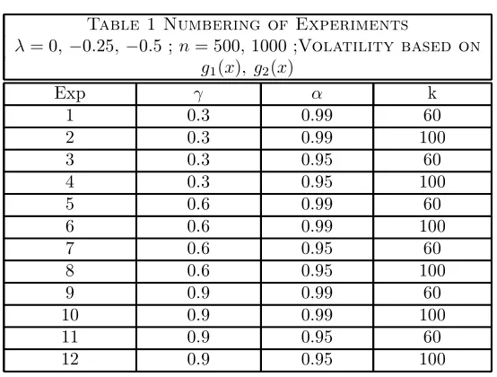
are two sample sizes considered for the ¯rst stage of the estimation nS =f500;1000g, three values for °, n° = _f0:3;0:6;0:9_g, three values for ¸, n¸ = _f0;_¡0:15;_¡0:5_g, two values for ®, n® = _f0:95;0:99_g, two values for the number of observations used in the second stage of the estimationk, nk=_f80;100_g, and two functional forms forg(x), which we denote byg1(x) = _1+exp(exp(¡_¡x)_x) andg2(x) = 1¡0:9exp(¡2x2). Graphs 1A and 1B in appendix 2 provide the general shape for these volatility speci¯cations together with that implied by GARCH type models. We now turn to the results of our Monte Carlo.

4 Results

We considered a total of nine estimators for VaR and TailVaR. There are four ¯rst stage estimators: the nonparametric method we propose, GARCH-N, GARCH-T, StAR; and two second stage estimators: the L-moments based estimator we propose and the ML estimator. In addition we consider a direct estimation method that estimates VaR and TailVaR assuming that²t in (11) is indeed distributed as an asymmetric Student-t density. In this case, all parameters are estimated via maximum likelihood. Since this direct ML estimator is based on a correct speci¯cation of the conditional density we expect it to outperform all other methods. Our focus is on the remaining estimators, which are all based on stochastic models that are misspeci¯ed relative to the DGPs considered. Speci¯cally, the nonparametric and StAR estimators are based on models in which the volatility function is assumed to depend only onYt_¡1 rather than the entire history of time series (markov property of order 1). The GARCH type models and StAR are misspeci¯ed in thatg in our DGPs is not linear inYt¡1. A summary of simulation results is provided in Appendix 2. G

G G

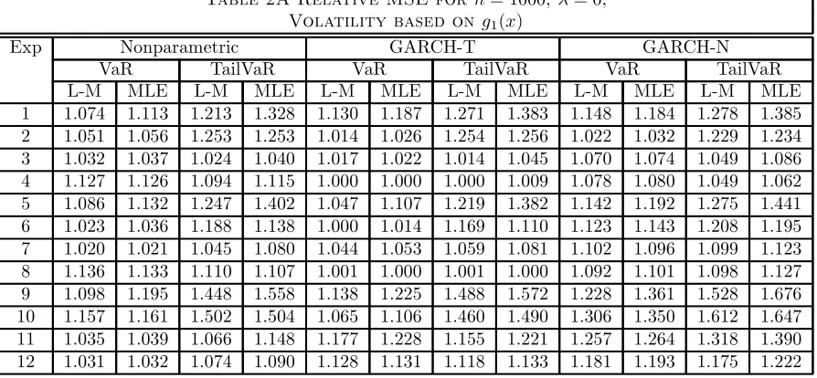
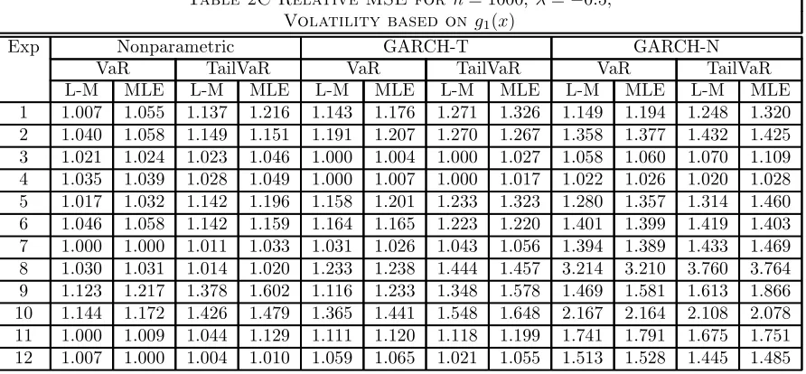
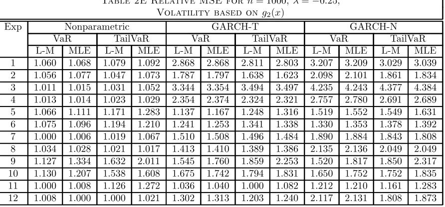
Geeenennenereerrraaaallll RRRReeseesssuuuullllttttss oss oononnn RRReRellllaeeaaattttiiiivvvvee Pee PPPeeererrrffffooroormrrmmamaaanncnnccceeee : Tables 2A-2F provide the ratio between an estimator's mean squared error(MSE) and the MSE for the direct estimation method forn= 1000, which we call relative MSE.7 _{As expected, in virtually all experiments, relative MSE>} _{1 indicating that the direct estimation} method (correctly speci¯ed DGP) outperforms all other estimators for VaR and TailVaR. More interestingly, 7_{Tables and graphs omit the results for the StAR method. This estimation procedure is consistently outperformed by all}

(16)

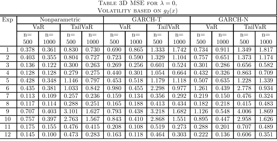
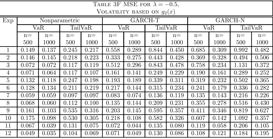
however, is that a series of very general conclusions can be reached regarding the relative performance of the other estimators:8 _{1) for both VaR and TailVaR estimation and all estimators considered, second stage} estimation based on L-moments produces smaller MSE than when based on ML. This conclusion holds for virtually all experiments, volatilities and ¸. The performance of ML based estimators seems to improve withk= 100 andn, but not signi¯cantly. 2) For DGPs based ong2, VaR and TailVaR estimators based on the nonparametric method produces lower MSE for virtually all experimental designs. Estimators based on GARCH-t are consistently the second best option. For DGPs based ong1, nonparametric based estimators of VaR and TailVaR outperform GARCH type methods in virtually all cases where°= 0:6;0:9. We detect no decisive impact of¸,n and other design parameters on the relative performance of the estimators.

These results generally indicate that the combined nonparametric/L-moment estimation procedure we propose is superior to GARCH/ML (and StAR) type estimators in virtually all experimental designs. Fur-thermore, since our estimator assumes thatfYtg is markov of order 1, contrary to GARCH type models, our results reveal that nonlinearities in volatility may be more important to VaR and TailVaR estimation performance then accounting for the non-markov property of the series. In fact, given thatg1(x) produces conditional volatilities that are similar to those empirically obtained in Hafner(1998), it seems warranted to conclude that this would indeed be the case for some typical time series of asset returns.9 We now turn to a discussion of the bias and MSE of the estimators.

R R R

Reeeessssuuuullllttttssss ooononnn MMMSMSESSEE aE aaannndnd BddBBiiiiaBaasasss : 1) Tables 3A-F show that MSE for VaR and TailVaR across all estimators falls with increasednfor virtually all design parameters and volatilities. There is, however, no distinguishable impact of increasingkon MSE for any of the estimators.10 _{This is most likely due to the range of}_k_{we have} used. 2) MSE for VaR and TailVaR estimators increases with the quantile across all design parameters and volatilities. 3) The impact of° on MSE is ambiguous for DGPs based on g2 and positive for g1 across all

8_{Unless explicitly noted conclusions are also valid for the cases when}_n_{= 500.}

9_{We found that in ¯nite samples, VaR and TailVaR estimators based on more sophisticated nonparametric estimators in the}

¯rst stage, such as that proposed by Carrol, HÄardle and Mammen(2002), did not outperform ours in ¯nite samples.

10_{Insensitivity of the GARCH-N/ML VaR estimator to changes in}_k_{in this range was also obtained in a simulation study by}

(17)

estimators and design parameters. 4) MSE for VaR and TailVaR estimators decrease signi¯cantly with¸ across all parameter designs and volatilities, specially when considering the nonparametric procedure. This is illustrated in Graphs 2A and 2B, where the ratioR= M SE(¸=_{M SE(¸=0)}¡0:5) <1. Since in our DGPs¸·0 the data is skewed towards the positive quadrant. For second stage estimation we are selecting data that are larger than thekth _{order statistic and considering the 95 and 99 percent quantiles. As such, more representative} data of tail behavior is used when ¸decreases. 5) The MSE across all design parameters, volatilities and estimators is signi¯cantly larger when estimating TailVaR compared to VaR. Hence, our simulations seem to indicate that the estimation of TailVaR is more di±cult than VaR, at least as measured by MSE. The result is largely due to increased variance in TailVaR estimation rather than bias.

The impact of various design parameters on the bias in VaR and TailVaR estimation across procedures, design parameters and volatilities is much less clear and de¯nitive than that on MSE. In particular, as the sample sizenorkincreases there is no clear impact on bias. Hence, the reduction on MSE whennincreases observed above is largely due to a reduction on variance. The most de¯nite result regarding estimation bias we could infer from the simulations is that all estimation procedures seem to have a positive bias in the estimation of VaR and TailVaR. Graphs 3A, 3B, 3C and 3D illustrate this conclusion forg1,g2,¸=¡0:25, n = 1000 for the best estimation methods, i.e., GARCH-T and the nonparametric method together with L-moment estimation. The exceptions seem to occur when° = 0:9, in which case there is negative bias.11 Although there are exceptions, in most DGPs the nonparametric method seems to have a slightly smaller bias than the other estimators.

5 Conclusion

In this paper we have proposed a novel way to estimate VaR and TailVaR, two measures of risk that have become extremely popular in the empirical, as well as theoretical ¯nance literature. Our procedure combines the methodology originally proposed by McNeil and Frey(2000) with nonparametric models of volatility

(18)

dynamics and L-moment estimation. A Monte Carlo study that is based on a DGP that incorporates empirical regularities of returns on ¯nancial time series reveals that our estimation method outperforms the methodology put forth by McNeil and Frey. To the best of our knowledge, this is the ¯rst evidence on the ¯nite sample performance of VaR and TailVaR estimators for conditional densities. It is important at this point to highlight the fact that asymptotic results for these types estimators are currently unavailable. In addition, results from our simulations seem to indicate that nonlinearities in volatility dynamics may be very important in accurately estimating measures of risk. In fact, our simulations indicate that accounting for nonlinearities may be more important than richer modeling of dependency.

References

1. AÄit-Sahalia, Y. and M.W. Brandt, 2001, Variable selection for portfolio choice. Journal of Finance, 56, 1297-1355.

2. Andreou, E., N. Pittis and A. Spanos, 2001, On modelling speculative prices: the empirical literature. Journal of Economic Surveys, 15, 187-220.

3. Artzner, P., F. Delbaen, J. Eber, J. and D. Heath, 1999, Coherent measures of risk. Mathematical Finance, 9, 203-228.

4. Basle Committee, 1996, Overview of the ammendment of the capital accord to incorporate market risk. Basle Committee on Banking Supervision.

5. Bollerslev, T., 1986, Generalized autoregressive conditional heterocedasticity. Journal of Econometrics, 31, 307-327.

6. Carroll, R.J., W. HÄardle and E. Mammen, 2002, Estimation in an additive model when the components are linked parametrically. Econometric Theory, 18, 886-912.

7. Chen, Yi-Ting, 2001, Testing conditional symmetry with an application to stock returns. Working Paper, Academia Sinica.

8. Christo®ersen, P., J. Hahn, and A. Inoue, 2001, Testing and comparing value-at-risk measures, Journal of Empirical Finance, 8, 325-342.

9. Diebold, F.X., T. Schuermann, J.D. Stroughair, 1998, Pitfalls and opportunities in the use of extreme value theory in risk management, in Advances in Computational Finance, A.-P. Refenes, J.D. Moody and A.N. Burgess eds., 2-12. Kluwer Academic: Amsterdam.

10. Ding, Z., C.W.J. Granger and R.F. Engle, 1993, A long memory property of stock market returns and a new model. Journal of Empirical Finance, 1, 83-106.

11. Diebolt, J. and D. Gu¶egan, 1993, Tail behaviour of the stationary density of general nonlinear autore-gressive processes of order 1. Journal of Applied Probability, 30, 315-329.

12. Embrechts, P., S. Resnick, and G. Samorodnitsky, 1999, Extreme value theory as a risk management tool. North American Actuarial Journal 3, 30-41.

(19)

14. Fan, J., 1992, Design adaptive nonparametric regression. Journal of the American Statistical Associa-tion, 87, 998-1004.

15. Fan, J. and Q. Yao, 1998, E±cient estimation of conditional variance functions in stochastic regression. Biometrika, 85, 645-660.

16. Gouri¶eroux, C., 1997, ARCH models and ¯nancial applications. Spriger: Berlin.

17. Haan, L. de, 1976, Sample extremes: an elementary introduction. Statistica Neerlandica, 30, 161-172. 18. Hafner, C., 1998, Nonlinear time series analysis with applications to foreign exchange volatility.

Physica-Verlag: Heidelberg.

19. Hansen, B., 1994, Autoregressive conditional density estimation. International Economic Review, 35, 705-729.

20. HÄardle, W. and A. Tsybakov, 1997, Local Polynomial estimators of the volatility function in nonpara-metric autoregression, 81, 223-242.

21. Hols, M.C.A.B. and C.G. de Vries, 1991, The limiting distribution of extremal exchange rate returns. Journal of Applied Econometrics, 6, 287-302.

22. Hosking, J.R.M., 1990, L-moments: analysis and estimation of distributions using linear combinations of order statistics. Journal of the Royal Statistical Society, B, 52, 105-124.

23. Hosking, J.R.M., 1987, Parameter and quantile estimation for the generalized pareto distribution. Technometrics, 29, 339-349.

24. Hosking, J.R.M. and J.R. Wallis, 1997, Regional frequency analysis. Cambridge University Press: Cambridge, UK.

25. Leadbetter, M.R., G. Lindgren, H. Rootz¶en, 1983, Extremes and related properties of random sequences and processes. Springer-Verlag: Berlin.

26. Longin, F., 2000, From value-at-risk to stress testing, the Extreme Value Approach. Journal of Banking and Finance, 24, 1097-1130.

27. Masry, E., 1996, Multivariate local polynomial regression for time series: uniform strong consistency and rates. Journal of Time Series Analysis, 17, 571-599.

28. Masry, E. and D. Tj¿stheim, 1995, Nonparametric estimation and identi¯cation of nonlinear ARCH time series: strong convergence and asymptotic normality. Econometric Theory, 11, 258-289.

29. McNeil, A.J. and R. Frey, 2000, Estimation of tail-related risk measures for heterocedastic ¯nancial time series: an extreme value approach. Journal of Empirical Finance, 7, 271-300.

30. Pagan, A. and G.W. Schwert, 1990, Alternative models for conditional stochastic volatility. Journal of Econometrics, 45, 267-291.

31. Patton, A.J., 2001, On the importance of skewness and asymetric dependence in stock returns for asset allocation. Working Paper, LSE.

32. Pickands, J., 1975, Statistical Inference Using Extreme Order Statistics,The Annals of Statistics, 3333

119-131.

33. Risk, 1999, Risk Software Survey. January, 67-80.

34. RiskMetrics, 1995, RiskMetrics Technical Document, 3rd Edition, JP Morgan.

(20)

36. Scaillet, O., 2002, Nonparametric estimation and sensitivity analysis of expected shortfall. Mathemat-ical Finance, forthcoming.

37. Smith, R.L., 1984, Threshold methods for sample extremes, in Statistical Extremes and applications, ed. Thiago de Oliveira, 621-638. Dordrecht: D. Reidel.

38. Smith, R.L., 1987, Estimating tails of probability distributions. The Annals of Statistics, 15, 1174-1207. 39. Shephard, M., 1996, Statistical aspects of ARCH and stochastic volatility models, in D.R. Cox, D.V. Hinkley and O.E. Barndor®-Nielsen, eds. Time Series Models in Econometrics, Finance and Other Fields, 1-67. London: Chapman and Hall.

40. Spanos, A., 2002, Student's t autoregressive model with dynamic heterocedasticity. Working Paper, Virginia Tech.

41. Tauchen, G., 2001, Notes on Financial Econometrics. Journal of Econometrics, 100, 57-64.

(21)

Appendix 1

whereB[®; ¯] is the beta function.

P Using the previous results we obtain the desired expression.

P

(22)

®3=

Simple manipulations yield,®3= 8·3

(23)

Appendix 2 - Tables and Graphs

Graph 1a conditional volatility based on g1(x)and GARCH Model

(24)

Graph 2a R=MSE(¸=_MSE(¸=0)¡0:5) onTailVaRusing L-Moments with n= 1000, Volatility based on g1(x) for GARCH-t, Nonparametric

(25)

Graph 3a Bias _£100 onVaR using L-Moments withn= 1000; ¸=¡0:25, Volatility based on g1(x) for GARCH-t, Nonparametric

(26)

Graph 3c Bias_£100 onVaRusing L-Moments with n= 1000; ¸=¡0:25, Volatility based on g2(x) for GARCH-t, Nonparametric

(27)

Table 1 Numbering of Experiments

¸= 0;¡0:25;¡0:5 ;n= 500;1000 ;Volatility based on g1(x); g2(x)

Exp ° ® k

1 0.3 0:99 60

2 0.3 0.99 100

3 0.3 0.95 60

4 0.3 0.95 100

5 0.6 0.99 60

6 0.6 0.99 100

7 0.6 0.95 60

8 0.6 0.95 100

9 0.9 0.99 60

10 0.9 0.99 100

11 0.9 0.95 60

(28)

Table 2A Relative MSE for n= 1000; ¸= 0; Volatility based ong1(x)

Exp Nonparametric GARCH-T GARCH-N

VaR TailVaR VaR TailVaR VaR TailVaR

L-M MLE L-M MLE L-M MLE L-M MLE L-M MLE L-M MLE

1 1.074 1.113 1.213 1.328 1.130 1.187 1.271 1.383 1.148 1.184 1.278 1.385 2 1.051 1.056 1.253 1.253 1.014 1.026 1.254 1.256 1.022 1.032 1.229 1.234 3 1.032 1.037 1.024 1.040 1.017 1.022 1.014 1.045 1.070 1.074 1.049 1.086 4 1.127 1.126 1.094 1.115 1.000 1.000 1.000 1.009 1.078 1.080 1.049 1.062 5 1.086 1.132 1.247 1.402 1.047 1.107 1.219 1.382 1.142 1.192 1.275 1.441 6 1.023 1.036 1.188 1.138 1.000 1.014 1.169 1.110 1.123 1.143 1.208 1.195 7 1.020 1.021 1.045 1.080 1.044 1.053 1.059 1.081 1.102 1.096 1.099 1.123 8 1.136 1.133 1.110 1.107 1.001 1.000 1.001 1.000 1.092 1.101 1.098 1.127 9 1.098 1.195 1.448 1.558 1.138 1.225 1.488 1.572 1.228 1.361 1.528 1.676 10 1.157 1.161 1.502 1.504 1.065 1.106 1.460 1.490 1.306 1.350 1.612 1.647 11 1.035 1.039 1.066 1.148 1.177 1.228 1.155 1.221 1.257 1.264 1.318 1.390 12 1.031 1.032 1.074 1.090 1.128 1.131 1.118 1.133 1.181 1.193 1.175 1.222

Table 2B Relative MSE forn= 1000; ¸=¡0:25; Volatility based ong1(x)

(29)

Table 2C Relative MSE forn= 1000; ¸=¡0:5; Volatility based ong1(x)

1 1.007 1.055 1.137 1.216 1.143 1.176 1.271 1.326 1.149 1.194 1.248 1.320 2 1.040 1.058 1.149 1.151 1.191 1.207 1.270 1.267 1.358 1.377 1.432 1.425 3 1.021 1.024 1.023 1.046 1.000 1.004 1.000 1.027 1.058 1.060 1.070 1.109 4 1.035 1.039 1.028 1.049 1.000 1.007 1.000 1.017 1.022 1.026 1.020 1.028 5 1.017 1.032 1.142 1.196 1.158 1.201 1.233 1.323 1.280 1.357 1.314 1.460 6 1.046 1.058 1.142 1.159 1.164 1.165 1.223 1.220 1.401 1.399 1.419 1.403 7 1.000 1.000 1.011 1.033 1.031 1.026 1.043 1.056 1.394 1.389 1.433 1.469 8 1.030 1.031 1.014 1.020 1.233 1.238 1.444 1.457 3.214 3.210 3.760 3.764 9 1.123 1.217 1.378 1.602 1.116 1.233 1.348 1.578 1.469 1.581 1.613 1.866 10 1.144 1.172 1.426 1.479 1.365 1.441 1.548 1.648 2.167 2.164 2.108 2.078 11 1.000 1.009 1.044 1.129 1.111 1.120 1.118 1.199 1.741 1.791 1.675 1.751 12 1.007 1.000 1.004 1.010 1.059 1.065 1.021 1.055 1.513 1.528 1.445 1.485

Table 2D Relative MSE forn= 1000; ¸= 0; Volatility based ong2(x)

(30)

Table 2E Relative MSE for n= 1000; ¸=¡0:25; Volatility based ong2(x)

1 1.060 1.068 1.079 1.092 2.868 2.868 2.811 2.803 3.207 3.209 3.029 3.039 2 1.056 1.077 1.047 1.073 1.787 1.797 1.638 1.623 2.098 2.101 1.861 1.834 3 1.011 1.015 1.031 1.052 3.344 3.354 3.494 3.497 4.235 4.243 4.377 4.384 4 1.013 1.014 1.023 1.029 2.354 2.374 2.324 2.321 2.757 2.780 2.691 2.689 5 1.066 1.111 1.171 1.283 1.137 1.167 1.248 1.316 1.519 1.552 1.549 1.631 6 1.075 1.096 1.194 1.210 1.241 1.253 1.341 1.338 1.330 1.353 1.378 1.392 7 1.000 1.006 1.019 1.067 1.510 1.508 1.496 1.484 1.890 1.884 1.843 1.808 8 1.034 1.028 1.021 1.017 1.413 1.410 1.389 1.386 2.135 2.136 2.049 2.049 9 1.127 1.334 1.632 2.011 1.545 1.760 1.859 2.253 1.520 1.817 1.850 2.317 10 1.130 1.207 1.538 1.608 1.675 1.742 1.794 1.831 1.650 1.752 1.752 1.835 11 1.000 1.008 1.126 1.272 1.036 1.040 1.000 1.082 1.212 1.210 1.161 1.283 12 1.008 1.000 1.000 1.021 1.302 1.313 1.203 1.240 2.117 2.131 1.808 1.873

Table 2F Relative MSE for n= 1000; ¸=¡0:5; Volatility based ong2(x)

(31)

Table 3A MSE for¸= 0; Volatility based ong1(x)