The Correlation Analysis of Exposure to the Electromagnetic Field
from Base Stations
Wanchun Yang*, Yongjun Liu, Bodong Li, and Chunhong Cao
Abstract—The effects of exposure to the electromagnetic field from base stations have received considerable attention. Currently, researches have shown that the exposure level from a base station varies with time due to the traffic. The traffic for mobile communications has a temporal and spatial correlation. In this paper, we develop an approach to study the variation law of exposure to the base stations and analyze the correlation of exposure in time and in space. We use a spectrum analyzer to measure the transmission power of the base stations at the different periods of a day. We obtain the analytical expressions for representing the variation of exposure with time using Genetic Algorithm. The self correlation of exposure to a single base station in time series and the cross correlation of exposure to base stations in the same area are both discussed. We find that the self correlation coefficients of exposure to a single base station are bigger than 0.9 in two hours and bigger than 0.5 in eleven hours. Particularly, the spatial correlation of exposure is slightly stronger than the time correlation, up to 0.99.
1. INTRODUCTION
With the rapid development of mobile communications, a large number of base stations are built around our residences. Potential risks for exposure to the electromagnetic field from these stations have attracted much attention from researchers [1–3].
The exposure level of the base station is not constant. It always changes with time because the traffic of base stations is variable in a day. To conduct an accurate assessment of exposure to the base station, recently many efforts are paid to study the variation of exposure with time. The actual exposure to the downlink channels, such as broadcast channel and traffic channels of the base station, was measured during a period of 24 h by a spectrum analyzer [4]. The results confirm that the traffic load has a great impact on the variation of the exposure level. The variation of exposure to the downlink channels of the base stations was measured on a daily, weekly and monthly basis by a SMP system and a selective radiation meter (SRM) 3006 [5]. It was found that the maximum and minimum electric fields are 2.36 and 1.18 V/m, respectively. In [6], exposure measurements were performed in the cities of Basel (Switzerland), Ghent and Brussels (Belgium), by an exposimeter of the type EME Spy 120 which can quantify exposure to the radio frequency electromagnetic field (RF-EMF) on 12 different frequency bands. The authors found that within one year, the total RF-EMF exposure levels in all outdoor areas in combination increased by 57.1% (p <0.001) in Basel, by 20.1% in Ghent (p = 0.053) and by 38.2% (p= 0.012) in Brussels. In [7], intensive measurements were conducted for 7 days at each of 7 different locations in urban area of Belgrade. The measurement results showed that the variation of exposure each day can be divided into two distinctive periods: one with the higher levels (9 h–23 h) and one with the lower ones (23 h–9 h) due to the traffic change.
Received 12 April 2016, Accepted 6 December 2016, Scheduled 22 December 2016
* Corresponding author: Wanchun Yang ([email protected]).
The variation of exposure is related to the traffic. The traffic not only has a temporal correlation, but also has a spatial correlation [8, 9]. However, the study for the self correlation of exposure to a single base station in time series and the cross correlation of exposure between base stations located in the same area is still absent until now. For example, in a residential area, during the day most of people leave this area to work. The electromagnetic exposure levels from multiple base stations will decrease simultaneously. But during the evening when people come home after work, the trends of the exposure to multiple base stations are all upward, which may lead to a sharp rise of exposure in an area. Due to the same living habits or lifestyle, the variation of exposure between the multiple base stations located in the same area has a strong correlation. This correlation is very important to accurately assess the exposure level of an area.
In order to analyze the correlation, in this work, we choose the base station of the third generation of mobile telephony (3G). These base stations always have only one transmitting channel with wide bandwidth. It is easy to track the real-time variation of exposure to these base stations by the spectrum analyzer in the zero-span mode. We measure the electric field radiated by these stations during 24 hours. The contribution of our work is that we obtain accurate expressions for the variation of exposure using Genetic Algorithm (GA). This algorithm applies the natural selection mechanism of the “survival of fittest” to eliminate the “Runge” phenomenon [15]. By these expressions, we analyze the self correlation of exposure to a single base station in the time series and the cross correlations of exposure between multiple base stations in the same area.
2. THEORETICAL MODEL
2.1. GA Model
In order to obtain the analytical expressions for the time-varying exposure to a base station, the algorithm GA was used in this paper. This algorithm uses the natural selection mechanism of the “survival of fittest” and can improve the accuracy of the expression. The expression for exposure with time can be established as
E(t) = m
i=1
aisin(bit+ci) (1)
where ai, bi, and ci are the parameters to be determined by GA, and t is the time. The following procedures are based on GA to determine the parameters ai,bi, and ci.
1). Input the measured electric filed strength at 24 hours of a day. The measured fields are denoted ase1,e2,. . ., and e24, respectively.
2). Encodeai,bi, and ci to get the initial population.
3). Compute E(t) at 24 hours by the values of ai,bi and ci. The calculated results is denoted as
E1,E2,. . ., and Ej,j= 1,2, . . . ,24.
4). Use the following Equations (2) and (3) to compute the fitness.
pj = (Ej−ej)2 (2)
p = n
j=1
(Ej−ej)2 (3)
pj is the individual fitness and pthe total fitness.
5). Genetic manipulation. We use three genetic operators: selection, crossover and mutation. 6). Set termination condition. If the condition is satisfied, then the model will output parameters
ai,bi, and ci. Otherwise the model will return to the step 4.
We use two metrics to evaluate the fitting goodness. The first one is the coefficient of determination, denoted as R-square. Ife1,e2,. . ., andenarenmeasured results andE1,E2,. . ., andEnarencalculated values, R-square is calculated as follows:
R-Square = 1−
n
j=1(Ej−ej) 2
n
j=1(Ej −¯e)
where ¯e is the mean value of{e1, e2, . . . , en}. R-square is in the range [0, 1]. If R-square is larger than 0.9, it indicates that the expression (1) is good enough to represent the measured results.
The second metric is root mean squared error (RMSE), which is defined as:
RMSE =
nj=1(Ej−ej) 2
n . (5)
The value of RMSE is set to be less than 0.02 in this paper for a small error between the expression and the measured exposure results.
2.2. Correlation Analysis
X and Y are denoted as two different base stations. EX(t) and EY(t) represent exposure toX and Y
at timet, respectively. The self-correlation coefficient of exposure to the base station is calculated as
pXX(τ) = RXX(τ)−u 2 X
σX2 (6)
whereuX and σX are the mean value and root-mean-square value ofEX(t), respectively. RXX(τ) is
RXX(τ) = lim T→∞
T
0
EX(t)EX(t+τ)dt. (7)
The cross correlation coefficient of exposure between base stations is calculated as
pXY(τ) = RXY(στ)−uXuY
XσY (8)
where
RXY(τ) = lim T→∞
1
T T
0
EX(t)EY(t+τ)dt (9)
3. MEASUREMENT RESULTS AND ANALYSIS
3.1. Measurement Scheme
The third generation of mobile telecommunications technology supports high speed data transmission and provides large capacity voice, high-speed data, image transmission and other services. At present, there are three kinds of mainstream technology standards: TD-SCDMA, WCDMA and CDMA2000 in the world [10]. In order to study the time-varying of electromagnetic radiation, we choose the student dormitory to conduct a week-long measurement, where the base stations for TD-SCDMA, WCDMA and CDMA2000 are all deployed, and the antennas of these stations are fixed on the same tower.
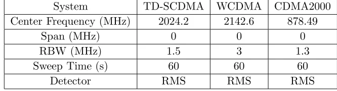
We measure exposure to the base stations by a spectrum analyzer in the zero-span mode during 24 hours. The exposure level for each hour is obtained by averaging the testing values of repeated measurements in that period. The settings of the spectrum analyzer are shown in Table 1 based on the methods in previous papers [10–13].
Table 1. Settings of the spectrum analyzer for the assessment of 3G exposure.
System TD-SCDMA WCDMA CDMA2000
Center Frequency (MHz) 2024.2 2142.6 878.49
Span (MHz) 0 0 0
RBW (MHz) 1.5 3 1.3
Sweep Time (s) 60 60 60
We convert the power (measured in dBm) intoE-field strength by
e= 10
⎡ ⎢ ⎢ ⎢ ⎢ ⎣−6+
20 lg ⎛ ⎜ ⎝
10(−3+10P)Z·106+AF+ARF ⎞ ⎟ ⎠
20
⎤ ⎥ ⎥ ⎥ ⎥ ⎦
(V/m) (10)
where the antenna factor (AF) is 22 dB/m, the power loss (ARF) of the cable which connects the antenna and the spectrum analyzer is 10 dB, and the input impedanceZ for this spectrum analyzer is 50 Ω.
3.2. Expressions for Exposure to the Base Stations
We measured exposure to base stations of TD-SCDMA, WCDMA and CDMA2000. Using GA, the expressions for the variation of exposure during the day are in the following.
ETD-SCDMA(t) = 0.087 sin (0.632t+ 0.596)−0.337 sin (1.298t−4.283)
−0.319 sin (−1.318t−1.819)−0.873 sin (−0.07t−0.491) (11)
EWCDMA(t) = 0.027 sin (0.666t+ 0.314)−0.189 sin (1.28t+ 2.142)
+0.657 sin (0.061t+ 0.664)−0.172 sin (−1.301t−1.906) (12)
ECDMA2000(t) = −0.83 sin (0.128t+ 3.745) + 0.013 sin (1.305t+ 3.604)
+0.188 sin (0.339t−1.484)−0.669 sin (−0.209t−3.109). (13)
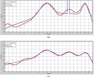
Figure 1 is the variation of exposure (i.e., the electric field strength) within 24 hours. The circles represent the measured results for 24 hours. The full lines are the results calculated from Eqs. (11), (12)
(a)
(c)
Figure 1. Exposure levels over 24 hours. (a) for TD-SCDMA; (b) for WCDMA; (c) for CDMA2000.
and (13), respectively. A Gaussian Mixture Model (GMM) is used to represent the variation of traffic of the base station [14]. The dotted line is calculated using GMM. Fig. 1 shows that the exposure increases at 8:00 and decreases at 23:00 due to the change of the traffic. From 8:00 to 23:00, the exposure is fluctuant in some periods of a day.
The biggest fluctuation is for exposure to TD-SCDMA in Fig. 1(a) because the exposure is related to the total transmitting power of the broadcast channel and service channels. The transmitting power of the service channel varies with the traffic. The transmitting power of the broadcast channel is always constant. But for TD-SCDMA using the code division multiplexing and time division multiplexing, the broadcast channel is transmitted only in a certain time slot. Compared with CDMA2000 and WCDMA, the average power of the broadcast channel is relatively low. Consequently, the fluctuation of exposure to TD-SCDMA is more obvious with the traffic.
From Table 2, the fitting accuracy of expressions based on GA is higher than that of expressions based on GMM. For example, in Table 2, R-square is 0.988 using GA, bigger than 0.964 using GMM. When using GMM, the “Runge” phenomenon [15] due to the round-off error appears in Fig. 1(a), which indicates that the GMM is not suitable for representing exposure to some base stations such as TD-SCDMA base stations where the variation of exposure is very large. The “Runge” phenomenon causes huge errors in fitting data. GA complies with the mechanism of natural selection through copy, crossover and mutation until we get the optimum solution. GA can achieve a better accuracy and avoid the “Runge” phenomenon.
Table 2. Fitting index for TD-SCDMA, WCDMA and CDMA2000.
GMM GA
TD-SCDMA
R-square - 0.979
RMSE - 0.017
WCDMA
R-square 0.964 0.988
RMSE 0.021 0.009
CDMA2000 R-square 0.968 0.990
3.3. Self Correlation
The variation of exposure is related to the traffic of the base station. The call arrival rate always exhibits a diurnal trend, with peak hours in the morning and late afternoon. The traffic has a strong temporal correlation. In the time series, the traffic flow of last moment can be regarded as a continuation of current traffic flow. The characteristics of the traffic demand for the same day in the same period are always similar.
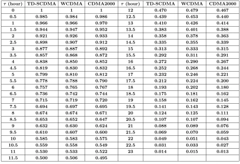
By substituting Eqs. (11), (12) and (13) into Eq. (6), the self-correlation coefficients of exposure to TD-SCDMA, WCDMA, and CDMA2000 were listed in Table 3. The correlation coefficients for three kinds of communication system have the same trend. They also show strong time dependence. For example, when τ is less than two hours, the correlation coefficients for three systems were very large, greater than 0.9. It indicates that when the exposure level begins to increase, the probability of the rise of exposure is very high in the coming two hours. When τ is larger than eleven hours, the coefficients were less than 0.5, indicating that the correlation in time series becomes weak after 11 hours.
Table 3. Self-correlation coefficients for TD-SCDMA, WCDMA and CDMA2000.
τ (hour) TD-SCDMA WCDMA CDMA2000 τ (hour) TD-SCDMA WCDMA CDMA2000
0 1 1 1 12 0.470 0.479 0.467
0.5 0.985 0.984 0.986 12.5 0.439 0.453 0.440
1 0.966 0.966 0.970 13 0.410 0.426 0.414
1.5 0.944 0.947 0.952 13.5 0.383 0.401 0.388
2 0.921 0.926 0.933 14 0.358 0.378 0.363
2.5 0.898 0.907 0.912 14.5 0.335 0.355 0.339
3 0.877 0.887 0.892 15 0.313 0.333 0.315
3.5 0.857 0.868 0.872 15.5 0.292 0.311 0.291
4 0.838 0.850 0.852 16 0.272 0.290 0.267
4.5 0.819 0.830 0.832 16.5 0.252 0.268 0.244
5 0.799 0.810 0.812 17 0.232 0.246 0.221
5.5 0.778 0.788 0.790 17.5 0.212 0.224 0.200
6 0.757 0.765 0.767 18 0.193 0.202 0.180
6.5 0.736 0.742 0.744 18.5 0.175 0.181 0.162
7 0.715 0.719 0.720 19 0.158 0.162 0.145
7.5 0.694 0.697 0.695 19.5 0.141 0.143 0.128
8 0.674 0.674 0.671 20 0.124 0.125 0.111
8.5 0.653 0.652 0.647 20.5 0.107 0.107 0.094
9 0.632 0.630 0.624 21 0.088 0.089 0.076
9.5 0.610 0.607 0.600 21.5 0.069 0.070 0.059
10 0.585 0.583 0.575 22 0.049 0.051 0.043
10.5 0.559 0.558 0.549 22.5 0.031 0.033 0.027
11 0.530 0.533 0.522 23 0.014 0.015 0.013
11.5 0.500 0.506 0.495
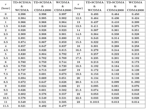
3.4. Cross Correlation
Table 4. Cross-correlation coefficients between TD-SCDMA, WCDMA and CDMA2000.
τ
(hour)
TD-SCDMA & WCDMA
TD-SCDMA & CDMA2000
WCDMA & CDMA2000
τ
(hour)
TD-SCDMA & WCDMA
TD-SCDMA & CDMA2000
WCDMA & CDMA2000
0 0.998 0.998 0.997 12 0.493 0.464 0.450
0.5 0.984 0.985 0.982 12.5 0.464 0.436 0.424
1 0.966 0.968 0.964 13 0.437 0.410 0.399
1.5 0.948 0.949 0.944 13.5 0.411 0.385 0.375
2 0.928 0.928 0.923 14 0.387 0.361 0.351
2.5 0.909 0.908 0.901 14.5 0.364 0.338 0.328
3 0.891 0.888 0.880 15 0.343 0.314 0.305
3.5 0.874 0.867 0.859 15.5 0.322 0.291 0.281
4 0.857 0.847 0.837 16 0.301 0.268 0.258
4.5 0.839 0.826 0.815 16.5 0.279 0.244 0.235
5 0.820 0.804 0.792 17 0.257 0.222 0.213
5.5 0.801 0.782 0.769 17.5 0.235 0.201 0.192
6 0.780 0.759 0.744 18 0.213 0.182 0.173
6.5 0.759 0.736 0.720 18.5 0.192 0.164 0.155
7 0.737 0.713 0.697 19 0.172 0.148 0.139
7.5 0.716 0.691 0.673 19.5 0.153 0.132 0.123
8 0.694 0.669 0.651 20 0.134 0.116 0.108
8.5 0.672 0.647 0.628 20.5 0.115 0.099 0..092
9 0.650 0.624 0.606 21 0.095 0.081 0.076
9.5 0.626 0.601 0.582 21.5 0.074 0.063 0.059
10 0.602 0.576 0.557 22 0.053 0.045 0.043
10.5 0.576 0.549 0.531 22.5 0.033 0.028 0.028
11 0.549 0.521 0.505 23 0.1015 0.013 0.014
11.5 0.521 0.492 0.477
communication systems is high degree of uniformity. When τ ≤11 hours, the correlation of exposure between the three systems is greater than 0.5. It indicates that when the exposure to one communication system increases, the exposure to the other two systems will quite possibly rise too. Particularly, the cross correlation coefficients between TD-SCDMA, WCDMA and CDMA2000 are slightly larger than the self correlation coefficients. For example, when τ = 0, the cross coefficients of exposure to base stations in the same area are up to 0.99. It shows that the spatial correlation of exposure is larger than the time correlation due to the same life-style. It is because the time correlation of exposure is dependent on the traffic. The traffic always fluctuates although it has a certain regularity. In contrast, the spatial correlation of exposure is dependent with the life-style. The life-style is more regular than the traffic, so that the spatial correlation is bigger than time correlation.
4. CONCLUSION
REFERENCES
1. Martens, A. L., J. F. Bolte, J. Beekhuizen, H. Kromhout, T. Smid, and R. C. Vermeulen, “Validity of at home model predictions as a proxy for personal exposure to radiofrequency electromagnetic fields from mobile phone base stations,” Progress In Environmental Research, Vol. 142, 221–226, 2015.
2. Plets, D., W. Joseph, K. Vanhecke, and L. Martens, “Exposure optimization in indoor wireless networks by heuristic network planning,” Progress In Electromagnetics Research, Vol. 139, 445– 478, 2013.
3. Beekhuizen, J., G. B. Heuvelink, A. Huss, A. B¨urgi, H. Kromhout, and R. Vermeulen, “Impact of input data uncertainty on environmental exposure assessment models: A case study for electromagnetic field modelling from mobile phone base stations,” Progress In Environmental Research, Vol. 135, 148–155, 2014.
4. Miclaus, S., P. Bechet, and C. Iftode, “The application of a channel-individualized method for assessing long-term, realistic exposure to radiofrequency radiation emitted by mobile communication base station antennas,” Measurement, Vol. 46, No. 3, 1355–1362, 2013.
5. Ozdemir, A. R., M. Alkan, and M. Gulsen, “Time dependence of environmental electric field measurements and analysis of cellular base stations,” IEEE Electromagnetic Compatibility Magazine, Vol. 3, No. 3, 43–48, 2014.
6. Urbinello, D., W. Joseph, L. Verloock, L. Martens, and M. R¨o¨osli, “Temporal trends of radio-frequency electromagnetic field (RF-EMF) exposure in everyday environments across European cities,” Progress In Environmental Research, Vol. 134, 134–142, 2014.
7. Koprivica, M., M. Petric, M. Popovic, J. Milinkovic, S. Niksic, and A. Neskovic, “Long-term variability of electromagnetic field strength for GSM 900 MHz downlink band in Belgrade urban area,”2014 22nd IEEE Telecommunications Forum Telfor (TELFOR), 9–12, 2014.
8. He, Q. Q., W. C. Yang, and Y. X. Hu, “Accurate method to estimate EM radiation from a GSM base station,” Progress In Electromagnetics Research M, Vol. 34, 19–27, 2014.
9. Hu, Z., Y. C. Chen, L. Qiu, G. Xue, H. Zhu, N. Zhang, and C. He, “An in-depth analysis of 3G traffic and performance,” Proceedings of the 5th Workshop on All Things Cellular: Operations, Applications and Challenges, 1–6, ACM, 2015.
10. Romero, J. P., O. Sallent, R. Agusti, and M. A. Diaz-Guerra, Radio Resource Management Strategies in UMTS, John Wiley & Sons, 2005.
11. Neskovic, N., M. Koprivica, A. Neskovic, and G. Paunovic, “Improving the efficiency of measurement procedures for assessing human exposure in the vicinity of mobile phone (GSM/DCS/UMTS) base stations,”Radiation Protection Dosimetry, ncr248, 2011.
12. Olivier, C. and L. Martens, “Optimal settings for narrow-band signal measurements used for exposure assessment around GSM base stations,” IEEE Transactions on Instrumentation and Measurement, Vol. 54, No. 1, 311–317, 2005.
13. Olivier, C. and L. Martens, “Optimal settings for frequency-selective measurements used for the exposure assessment around UMTS base stations,” IEEE Transactions on Instrumentation and Measurement, Vol. 56, No. 5, 1901–1909, 2007.
14. Nan, E., X. Chu, W. Guo, and J. Zhang, “User data traffic analysis for 3G cellular networks,”
2013 IEEE Conference on 8th International ICST Communications and Networking in China (CHINACOM), 468–472, 2013.