Multi-chain algorithm for wireless sensor networks based on
energy balance
QiChao TangP *
P
,MengLu SunP *
*Chongqing Key Lab of Mobile Communications Technology, Chongqing University of Posts and Telecommunications, Chongqing 400065, P. R. China
Abstract
The research of hierarchical algorithm is an effective method to prolong the network lifetime in wireless sensor networks. Multi-Chain algorithm for wireless sensor networks based on energy balance(MECB) is proposed to improve the time driven wireless sensor system which has a higher requirement for timeliness. Firstly, by using static clustering, each sub-region selects its leader node and then establishes the link with the leader node according to the path loss and gradient. Finally, a root node is selected by jointly taking account of the degree of node, the residual energy and the distance from the base station. In the process of link reconfiguration, the network performance is improved by controlling the recombination frequency of the controlled nodes. Finally, MECB algorithm can achieve the low network delay and high network lifetime.
Keywords: Wireless sensor networks, hierarchical algorithm, gradient, network lifetime, path loss
1. Introduction
Wireless sensor networks(WSNs) is a multi-hop self-organizing network system formed by a large number of sensor nodes deployed in the monitoring area. It is an important technical form of the underlying network of Internet of ThingsP
[1]
P
. In recent years, wireless sensor networks have been widely used in environmental monitoring, target tracking and battlefield detection because of the advantages of self-organization, rapid deployment, high fault tolerance and strong concealment. But once the node’s energy is exhausted, it can’t be added. Because sensor nodes are usually located in a dangerous environment, charging or replacing a battery is generally
unrealistic. So how to save energy and prolong network life is a question that need to be solved. For time driven wireless sensor system ,it not only requires low energy, but also requires a low network delay.
In order to solve these problems, many scholars and experts put forward a variety of energy-saving strategies. Especially Hierarchical routing protocol for WSNs is used widely, its main areas include: link-based, Grid-based, region-based, etcP
[1]
P
. The protocol based on link is the most extensive among them.
As the typical link-based protocol, PEGASIS has some shortcomings: a. it may lead to the long chain between adjacent nodes; b. the method selecting the leader may cause that energy consumption is not balanced; c. the re-election frequency of leader increases the communication overheadP
[2]
P
.
Energy Efficient PEGASIS-Based Protocol(EEPB) reduce the production of long chain by introducing distance thresholds. In this algorithm, the node selection is based on the residual energy of nodes and the distance from the node to the base station. But there is a problem that the size of the threshold is not easy to be determined. A Multi-Chain based Hierarchical Topology Control Algorithm for Wireless Sensor Networks(MCHTC)P
[3]
P
has some shortcomings: a. it has some problems in energy analysis ;b. There is a certain network delay.
Based on the above problems, this paper presents Multi-chain algorithm for wireless sensor networks based on energy balance(MCEB). The theoretical analysis and simulation results show that MCEB is better than LEACH, PEGASIS and MCHTC, it can lead to the better network lifetime and network latency.
2. The system model of MCEB
2.1 system hypothesis
1) N sensor nodes are randomly distributed in the monitoring area, and the BS is located far away from the monitoring area;
2) once the sensor nodes with the same finite initial energy are deployed, they will be in a static state. BS having the infinite energy is fixed;
3) communication link is symmetrical. Node SRi Rcan
communicate with the node SRj Rand node SRjR can
communicate with the node SRi R;
4) The sensor node can know its own location information by positioning technology. They can calculate the distance with communication node through the signal strength;
2.1 energy consumption model
Fig.1 is the energy consumption model of wireless sensors. Energy consumption model only considers the energy consumption of data transmission and data aggregation. The first consists of two parts: the loss of transmitter circuit and power amplificationP
[4]
P
.
Transmitter Amplifier Receiver
d
K bit packet K bit packet
Fig.1 Energy consumption model of wireless sensors
The energy consumed in sending k bit data packet over a distance d for each node is as in Eq.(1).
_ ( ) _ ( , )
2 0
4 0 ( , )
,
,
TX TX elec k TX amp k d
elec fs elec mp
E k d E E
kE k d d d
kE k d d d
ε ε
= +
+ <
= + ≥
(1)
where
E
elecis the energy consumed in electronics, d is thedistance between the transmitter and receiver, dR
0R is the
reference distance satisfying d0 =
ε ε
fs mp .If0
d
<
d
,power amplifier uses the free space loss model;If
d
≥
d
0, power amplifier uses the multi-path fadingmodel.
ε
fs andε
mpare the energy consumed in amplifiers.The energy consumed in receiving k bit data packet is as in Eq.(2).
( , )
RX elec
E
k d
=
kE
(2)The energy consumed in aggregating x data packet to a single packet is as in Eq.(3).
E
fuse x k( , )=
xkE
DA (3)where
E
DAis the energy parameters in Data fusion .3. MCEB protocol
The algorithm is based on t rounds and each round is divided into four phases, including sub-region division phase, sub-regional link formation phase, link of leader node formation phase, as well as the data transmission phase.
The sensor nodes are divided into sub-regions, and the sensor nodes
join different clusters
Create a link in each sub-region and select the leader node
Create links between the leader nodes and select
the root node start
leader node?
The root node communicates directly
with the base station
end
normal node N
Y Network
initialization
The base station obtains information such as node id,
location, and so on
root node? leader node
Y N
Fig.2 Algorithm flow chart
1) sub-region division phase
frameSin _k Sys Msg N R r_ ( , , ) to all other nodes in the
sensor network in a flooding manner, where N is the total number of nodes, R is the monitoring area radius, and r is the communication radius of the node. All nodes in the monitoring area learn their own distance to the base station according to their own location information pos and the
message Sin _k Sys Msg_ , then classify level according
to these distance information, level calculation is as in as in Eq.(4).
0
( )
(
dist
toBS)
level i
ceil
d
=
(4)where disttoBSis the distance between node i and BS, d
R
0R is
the reference distance.
The algorithm divides the network area into m regions in the horizontal and vertical direction. Once these regions are divided, they will no longer change and realize static clustering in the whole life cycle of the network. The number of optimal sub-regions can obtain according to the network energy balance EB . EB is as in Eq.(5).
0
2 0 1
(
)
N
i av
i
EB
ld
ld
N
=
=
∑
−
(5)where ldi is the factor of node energy load , ldav is the
factor of average energy load , NR
0R is the number of
sensor nodes.
EB
shows that the smaller the gap betweeni
ld and the ldav, the more balanced energy consumption of
the node, and the more reasonable sub-region division isP[5]P.
2) sub-regional link formation phase
From the farthest sensor node , link formation is based
on the distance energy ED i j( , ).ED i j( , )is as in Eq.(6).
0( )
( , ) ( , ) * ( )
r
E j
ED i j Ploss i j
E j
= (6)
where Ploss i j( , )is the path loss between node i and node
j,E0( )j is the initial energy of node j,Er( )j is the residual
energy of node j. Path lossPloss i j( , ) is as in Eq.(7).
Ploss i j( , )= p it( )−rssi j( ) (7)
where p it( ) is the sending signal strength of node
i ,rssi j( )is the receiving signal strength of node j.
In each sub region, the node having the furthest distance from the base station begins to create link according to distance energy. At the beginning of each round, the algorithm set an average residual energy. As long as the energy of the node is above over average residual energy, the node becomes the candidate cluster head node . Then from these nodes, choose the node having the nearest distance from the base station to be leader node. Average residual energy is as in Eq.(8).
0
1
(
)
av each
E
NE
E
N
=
−
(8)where N is the number of sensor nodes,E0is the initial
energy of per sensor node, Eeachis the consumed energy in
a per round.
3) link of leader node formation phase
start
is minimum?
( , )
ED i j
{ }
S= i G= −V { }i
{ , }
S= i jG= −V { , }i j
( , )
w k i
i∈S
is minimum?
{ , , }
S= i j k
{ , , }
G= −V i j k
Choose node k
{ }
G= φ ?
end Choose the node i that
is fastest from BS
Y Choose the node
i from G
Y Choose node i
Y
N
N N
i∈G k∈G
Fig.3 Flow chart of leader node link
the fastest distance from the BS choose the node j from V,
making ED i j( , ) is minimum. Then according to the
distance between the node and BS, the node from far to near joins the link. Assume the node k that is waiting for joining the link, the link k choose the minimum
Competition weight
w k i
( , )
, where i∈S .Finally thewhole leader nodes form structure named tree.
w k i
( , )
isas in Eq.(9).
( , )
( , )
(1
)
( )
( )
r
Ploss k i
w k i
a
a level i
E i
=
+ −
(9)where Ploss k i( , )is the consumed energy between node k
and node i , E ir( ) is the residual energy of node i,
( )
level i can obtain from Eq.(4).
From the link consists of the whole leader nodes, we can select the root node according to scaling function Q, Q is as in Eq.(10).
( )
( )
( ) *
r
toBS
E i
Q i
i
d
ρ
=
(10)where E ir( )is the residual energy of node i,dtoBS is the
distance between the node i and BS,
ρ
( )
i
is the ratio of the total number of physical neighbor nodes within communication radius of the node i to the communicationarea of the node i.
ρ
( )
i
is as in Eq.(11).2
_
( )
( )
i
neighbor
alive i
r
ρ
π
=
(11)where neighbor_alive i( )is the total number of physical
neighbor nodes within communication radius of the node i, r is the communication radius of node I. [6]
According to Eq.(10), we can see that the node having few physical neighbor nodes, the high remaining energy, short distance between the node and the base station is more easier to become the root node.
4) data transmission phase.
In the data transmission phase, from the end of the chain, the node transmits the collected data to the next hop neighbor node. The neighbor node combines its own data with the received data and sends it to its neighbor node until it reaches the root node. Root node goes data fusion collected and send the packet to the base station directly to complete a round of communication.
Control link reconfiguration frequency by proportional function round, round is as in Eq.(12).
max
*
cur each
cur ini
r
E
round
r
r
E
=
=
(12)where rcuris Current work rounds of the network, rmaxis
the max works rounds of the network.
In the first few rounds, because of the sensor nodes have sufficient energy, don’t carry out repeated election of leader nodes in the sub region, maintaining the leader node link unchanged. When round>0.5, election of leader nodes is selected for each round, causing the leader node link reorganization. This method can avoid the energy loss due to excessive restructuring.
4. Simulation experiment and result analysis
This paper uses the MATLAB platform to further analysis of the performance of MCEB algorithm, and compared its performance with the LEACH algorithm, PEGASIS algorithm and MCHTC algorithm.
4.1 performance parameters of the algorithm
1) the number of node alive: the number of node alive can direct reflect the life of network in WSNs. The more network nodes of survival in each round, indicate that the stronger of network life.
2) the residual energy of network: network life only reference node number of survival is not fully reflect the performance of network, the network life is negatively related to the consumption of energy, the greater the energy consumption, the shorter the network lifetime, whereas the longer.
4) network survival time: the network lifetime of wireless sensor network refers to the time by the end of the first node death.
4.2 The simulation scenario settings
100 nodes randomly distributed in square area which’s the side length is 100m, these nodes are fixed in the entire network life cycle after they are deployed. The base station in the outside of monitoring area, the coordinates is(50,150). The simulation parameters as shown in Table 1.
Table 1:simulation parameters
Simulation parameters value
the size of network 100×100
number of nodes 100
The location of BS (50,150)
size of packet 4000 bit
the length of control message 100 bit
fs
ε 100 pJ/bit/mP
2
mp
ε 0.0013 pJ/bit/mP
4
DA
E 5 nJ/bit/signal
initial energy of node 0.5J
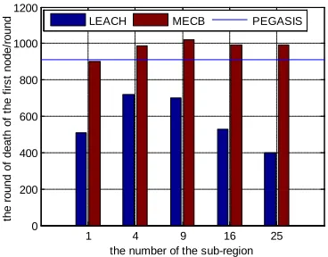
For some time driven sensor networks with high timeliness requirement, the sensors collect data periodically and send to the sink node, and the data acquisition and transmission are processed according to the pre-set schedule. For the same piece of monitoring area, the number of sub regions selected in MCEB algorithm would have a great influence on the survival time of the network. Through the simulation results in figure 4 and figure 5, it shows that when the monitoring area is divided into 9 regions, the survival time of the network and the network energy balance effect are both good. Thus, this paper will divide the monitoring area into 9 regions as in the following simulations. In the simulation experiment, Fig.6 shows the topology of wireless sensor network. The base station is located at (50,150), and the monitoring area is divided into nine sub-regions.
Fig.4 The relationship between the number of death round and the
number of the sub-region
Fig. 5 The relationship between the network energy balance and the
number of sub-region
Fig.6 Topology of wireless sensor networks
1 4 9 16 25
0 200 400 600 800 1000 1200
the number of the sub-region
the r
ound of
deat
h of
t
he f
ir
s
t node/
round
LEACH MECB PEGASIS
1 4 9 16 25
0 0.05 0.1 0.15 0.2
the number of the sub-region
net
w
or
k
l
if
et
im
e
LEACH
improve multi-chain PEGASIS
0 20 40 60 80 100
4.2 Simulation analysis
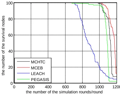
Fig. 7 Comparison of the number of survival nodes of different
algorithms
From Fig.7, we can see that compared with LECH,PEGASIS protocol, the round of the death time of the first node is obviously much behind, because of Path loss, node gradient, recombination frequency. Compared with MCHTC protocol, the round of the death time of the first node is also behind. The main reason for this situation is that considers recombination frequency and density of neighbor node.Through Table 2, we can see the effect of the recombination frequency on the death number of nodes. Compared with the MCEB algorithm without the control of the recombination frequency, death rounds of the nodes using the MCEB algorithm with the control of recombination frequency is obviously lagging behind .
Table 2: The effect of recombination frequency on the number of node deaths
MCEB protocol 10% node death / round
50%node death / round without the control of the
recombination frequency 1028 1111 with the control of
recombination frequency 1096 1186
It can be seen from Figure 8, because of classic LEACH algorithm using single-hop transmission classic LEACH algorithm, each round of the transmission time is the shortest, however, the transmission time of PEGASIS is the longest by using of single-link. MCEB algorithm and MCHTC algorithm adopt the way of dividing the
sub-region, reduce the long-chain generation and shorten the network delay. And the transmission delay of MCEB algorithm is significantly smaller because of level, which makes data fusion happened near from the basic station.
Fig. 8 Comparison of each round of transmission time in different
algorithms
Fig.9 reflects the relationship between the total residual energy of the sensor node and the number of simulated rounds. It can be seen from the Fig.9 , LEACH algorithm uses the single-hop communication to make the residual energy of the sensor node decline fast. And the residual energy of PEGASIS is not ideal because of considering insufficient. Compared to the MCHTC algorithm, the remaining energy of MCEB algorithm with the increasing number of simulation rounds, the decreasing speed is relatively slow, because of taking the path loss of the node into account in the process of selecting the next hop. is taken The improved MCEB algorithm also considers of recombination frequency of node.
Fig. 9 Comparison of residual energy of different algorithms
0 200 400 600 800 1000 1200 0
20 40 60 80 100
the num
ber
of
t
he s
ur
v
iv
al
nodes
the number of the simulation rounds/round MCHTC
MCEB LEACH PEGASIS
150 200 250 300 350 400 450 0
0.005 0.01 0.015 0.02 0.025 0.03 0.035
eac
h r
ound of
t
he t
rans
m
is
s
ion t
im
e/
s
Number of simulation rounds/round PEGASIS MCHTC IMCHR LEACH
0 200 400 600 800 1000 1200 0
10 20 30 40 50
the r
es
idual
ener
gy
/J
5. Conclusions
This article introduced MCEB algorithm According to four aspects. sub-region division phase, sub-regional link formation phase, link of leader node formation phase and the data transmission .The algorithm of mentioned in this article is mainly in the leader node linking phase, which takes into account the link of the restructuring frequency, the root node election factors and the choice of the next-hop. According to experiment simulation, the result prove that MCEB algorithm has lower network latency and better network lifetime, and the network energy balance get improved obviously. This is more important to some time driven sensor networks with high timeliness requirement.
Acknowledgments
This work was supported in part by the Program for Changjiang Scholars and Innovative Research Team in University (IRT1299),Project of CSTC (CSTC2012jjA40044, CSTC2013yykfA40010)and special fund of Chongqing key laboratory (CSTC).
References
[1] LIU Xu. A typical Hierarchical Routing Protocols for Wireless
Sensor Networks: A Review [J]. IEEE Sensor Journal,2015,15(10):
5372-5383.
[2] Lindsey S, Raghavendra C S. PEGASIS: Power-efficient gathering in
sensor information systems[C]//Aerospace Conference Proceedings.
IEEE,2010:1125 -1130.
[3] TANG Hong, WANG Hui-zhu. A Multi-Chain Based Hierarchical
Topology Control Algorithm for Wireless Sensor Networks[J]. Ksii
Transactions on Internet & Information Systems, 2015, 9(9):3468-3495
[4] SUN Yang, HE Jian-zhong. Adaptive load-balancing clustering
hierarchical routing protocol for WSN[J]. Computer Engineering and
Design, 2013, 34(2):423-427.)
[5] TANG Qiang, et al. Semi-centralized Clustering Protocol with
Energy Balance and Multi-hop Transmissions[J]. Journal of Chinese
Computer Systems, 2010, 33(4):583-586.
[6] YIN Xi, LI Zhihua, SUN Ya, et al. Network clustering topology
control algorithm based on node competitiveness [J]. Computer
Engineering and Applications, 2015, 51(8):79-84.
Qichao Tang, was born in Weihai of Shandong province in 1989.
He is now a graduate student in Chongqing University of Posts
and Telecommunications. His research concerns Wireless sensor
network.
Menglu Sun, was born in Pingdingshan of Henan province in
1992. She is now a graduate student in Chongqing University of Posts
and Telecommunications. Herresearch concerns mobile communication