VHDL Implementation of An Area Efficient Algorithm for Turbo
Decoders having Wireless Sensor Networking Applications
SHAHIDA T A1, ANU PHILIP MATHEW2
1
M-Tech student, ECE Department, Mangalam College of Engineering,
Kottayam, Kerala, India
2
Assistant Professor ECE Department, Mangalam College of Engineering,
Kottayam, Kerala, India
Abstract
Forward-error-correcting (FEC) channel codes are commonly used to improve the energy efficiency of wireless communication systems. The use of turbo codes enhances the data transmission efficiency in digital communications systems especially for wireless communication systems. In this paper, an area efficient Constant Log MAP Algorithm is introduced for turbo decoder and it is compared with LUT Log MAP algorithm. The simulation results shows that turbo decoder simulated using constant Log MAP algorithm requires less area and hence less power consumption. The simulation of turbo encoder using flip flop method and decoder using constant Log MAP algorithm makes this decoder more efficient.
Keywords: Look Up Table (LUT), Maximum A Posteriori (MAP), Log Likelihood Ratio (LLR), iterative decoding, interleavers.
1. INTRODUCTION
Turbo coding is a very powerful error correction technique that has made a tremendous impact on channel coding in the last few years. It outperforms all previously known coding schemes by achieving efficient error correction using simple component codes and large interleavers. The iterative decoding mechanism, recursive systematic encoders and use of interleavers are the characteristic features of turbo codes. The use of turbo codes enhances the data transmission efficiency in digital communications systems. This technique can also be used to provide a robust error correction solution to combat channel fading. The entire turbo coding scheme consists of recursive systematic encoders, interleavers, puncturing and the decoder. This paper gives a brief overview of the various components of the turbo coding scheme, analyzes the complexities of the most popular turbo decoding algorithms, describes a suitable model of computation and
discusses the various implementation methods of the maximum a posteriori (MAP) algorithm.
2. TURBO CODING SYSTEM
In wireless sensor networks, for reliable data transmission, the data need to be encoded at the transmitter and then decoded at the receiver. So a turbo coding system consists of turbo encoders, interleavers and turbo decoders. The input data first enters the turbo encoder. From the turbo encoder, the encoded data passes through the noisy channel, then to the turbo decoder. The turbo decoder produces the decoded output.
2.1 TURBO ENCODER AND INTERLEAVER
The general structure of a turbo encoder is shown in Fig. 1. It consists of two rate half Recursive Systematic Convolutional (RSC) encoders C1 and C2. The N bit data block is first encoded by C1. The same data block is also interleaved and encoded by C2.The main purpose of the interleaver is to randomize bursty error patterns so that it can be correctly decoded
The interleaver is a very important constituent of the turbo encoder. It spreads the bursty error pattern and also increases the free distance. Thus, it allows the decoders to make uncorrelated estimates of the soft output values. The convergence of the iterative decoding algorithm improves as correlation of the estimates decreases.
the number of bits (or quantization) selected as the output of each decoder. The deinterleaver performs the opposite function of the interleaver; where the interleaver permutes the data, the deinterleaver de-permutes the data back to the original order.
Fig. 1 Turbo Encoder
Fig. 2 RSC Encoder
2.2TURBO DECODER
A turbo decoder comprises a parallel concatenation of two decoders, that employ different types of decoding algorithms. Rather than operating on bits, each decoder processes Logarithmic Likelihood Ratios (LLR) where each LLR=ln((P(b=0))/P(b=1))) quantifies the decoder’ s confidence concerning its estimate of a bit from the bit sequences. Different algorithms are used for turbo
decoders. The algorithm that is used in turbo decoder is maximum a posteriori (MAP) algorithm. There are different versions of MAP algorithm. Based on the algorithm used, the area required and power consumed by the turbo decoder varies.
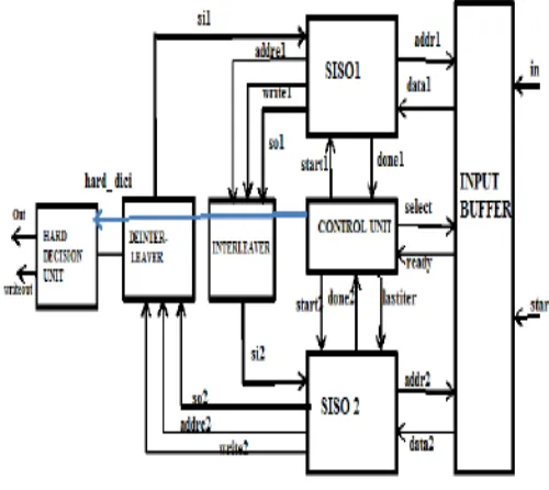
The encoded data that passes through the noisy channel enters the input buffer. Input buffer stores the received information. The 2 blocks of data enters SISO 1 and SISO 2. When the control module sends the signal START_SISO1, SISO 1 starts the iteration. Inside SISO 1 the LLR value corresponding to each bit is calculated using the algorithm.
Once it completes the first iteration, it sends back DONE_SISO1 signal to control module. This makes control module to send the START_SISO2 signal and SISO 2 starts the iteration. The input of SISO 2 is data from input buffer and the output of SISO 1 after passing through the interleaver. Once SISO 2 completes the iteration, it sends DONE_SISO2 signal to the control module. Similarly the input to SISO 1 is data 1F and data 1B from input buffer and the output of SISO 2 after passing it through deinterleaver. The SISO 1 and SISO 2 modules perform the iteration using the algorithm. During the iteration, parameters like α, β, γ are calculated. The final output is taken from the deinterleaver after a particular number of iteration. The final output will also be LLR values. If this LLR value obtained is negative then it will be decoded as 1 and if it is positive it is decoded as 0.
3. MAXIMUM A POSTERIORI
ALGORITHM
The process of turbo-code decoding starts with the formation of a posteriori probabilities (APPs) for each data bit, which is followed by choosing the data-bit value that corresponds to the maximum a posteriori (MAP) probability for that data bit. Upon reception of a corrupted code-bit sequence, the process of decision making with APPs allows the MAP algorithm to determine the most likely information bit to have been transmitted at each bit time.
3.1 CONVENTIONAL LUT LOG MAP ARCHITECTURE
Conventional LUT-Log-MAP architecture, which employs the sliding-window technique to generate the LLR sequence as the concatenation of equal length sub-sequences. Each of these windows is generated separately, using a forward, a pre-backward and a backward recursion.
In turbo decoder, the SISO modules undergo a number of iteration using the algorithm. During the iteration certain parameters like α, β, γ are calculated. γ is branch metrics. α and β are node metrics. Using γ, the node metrics α and β are calculated.
γ = 0.5 exp (xk uk + yk vk) (1)
α k+1 (s‘) = max* s to s‘ (αk (s) + Σi=1 to 2 γ (s,s‘) (2)
β k-1 (s) = max* s to s‘ (αk (s‘) + Σi=1 to 2 γ (s,s‘) (3)
to obtain the values of α and β max* operation is required. This operation is performed using MAP algorithm.
3.2 LUT Log MAP Algorithm
Max*(x,y)=max(x,y) + 0.75, if |y-x|=0
0.5, if |y-x|=(0.25,0.5,0.75)
0.25,if |y-x|=(1,1.25,1.5,1.75,2) (4)
4. PROPOSED CONSTANT LOG MAP
ALGORITHM
This is another version of MAP algorithm. To determine node metrics (α, β) during SISO iteration, max* operation is required. The max* operation associated with constant Log MAP algorithm is as follows.
Max*(x,y ) = max(x,y) + 0, if |y-x|>T
C, if |y-x|<=T (5)
Where T=1.5, C=0.5
In this max* operation after obtaining maximum of x and y, based on the range of |y-x| correction factor 0.5 is added.
So, compared to LUT Log MAP algorithm, this is a low complexity algorithm. In it, we can take a threshold value, T and based on that value, we can add correction factor C. In this paper, T is taken as 1.5 and C is taken as 0.5.
5. RESULTS
Turbo encoder and turbo decoder are simulated using ModelSim 6.4a and implemented in Xilinx Virtex6 FPGA. The synthesis report shows that Turbo decoder using Constant Log MAP algorithm has less usage of hardware resources and less power than that using LUT Log MAP algorithm.
Fig. 4 Synthesis report showing power consumption of LUT Log MAP Decoder
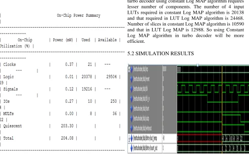
Fig.5. Synthesis report showing power consumption of Constant Log MAP Decoder
Table.1.Device utilization summary of LUT Log MAP decoder and Constant Log MAP decoder
Logic Utilization
LUT Log MAP Decoder
Constant Log MAP
Decoder
Available
Number of
slice registers 2358 2346 29504 Number of
flip flops 2055 2043 -
Number of
latches 303 303 -
Number of 4
input LUTs 24468 20138 29504
Number of
slices 12988 10590 14702
Number of
bonded OBs 10 10 250
The device utilization summary of LUT Log MAP algorithm and constant Log MAP algorithm shows that turbo decoder using constant Log MAP algorithm requires lesser number of components. The number of 4 input LUTs required in constant Log MAP algorithm is 20138 and that required in LUT Log MAP algorithm is 24468. Number of slices in constant Log MAP algorithm is 10590 and that in LUT Log MAP is 12988. So using Constant Log MAP algorithm in turbo decoder will be more efficient.
5.2 SIMULATION RESULTS
Fig.7. Simulation result of Constant Log MAP Decoder
4. Conclusions
In this paper, turbo coding is simulated using ModelSim 6.4a and implemented in Xilinx Virtex6 FPGA. Turbo encoder is implemented by using flip flops as memory elements. Turbo Decoders are performed by LUT Log MAP algorithm and Constant Log MAP algorithm. Synthesis report shows that turbo decoder using Constant Log MAP Algorithm have low power and less area utilization than that using LUT Log MAP algorithm.
References
.[1] Liang Li, Robert G. Maunder, Bashir M. Al-Hashimi, "A low-complexity turbo decoder architecture for energy-efficient wireless sensor networks", IEEE, Vol. 21, No. 1, 2013,pp.1063-8210
[2] S. L. Howard, C. Schlegel, and K. Iniewski " Error control coding in low-power wireless sensor networks:When is ECC energy-efficient?,", EURASIP J. Wirel. Commun. Netw., vol. 2006, pp. 1–14, 2006.
[3] I. F. Akyildiz, W. Su, Y. Sankarasubramaniam, and E. Cayirci"
Wireless sensor networks: A survey,", Comput. Netw.:
Int. J. Comput.Telecommun. Netw., vol. 52, pp. 292–
422, 2008.
[4] C. Schurgers, F. Catthoor, and M. Engels" Memory optimization of
MAP turbo decoder algorithms,", IEEE Trans. Very Large Scale Integr.(VLSI) Syst., vol. 9, no. 2, pp. 305–312, Feb. 2001.
SHAHIDA T A received BTech degree in Electronics and Instrumentation Engineering from College of Engineering, Kidangoor , Kottayam, Kerala, India in 2010 and pursuing MTech in VLSI And Embedded system in Mangalam College Of Engineering, Kottayam, Kerala., India.