Short communication:
An interpretation of the Linux entropy estimator
BenjaminPousse
benjamin(dot)pousse(at)gmail(dot)com
Institute: None
Abstract. The Linux [1] random number generator (LRNG) aims to produce random numbers with all the limitations due to a deterministic machine. Two recent analysis exist for this generator [2,5]. These analysis provide strong cryptographic details about LRNG. However both fail to give a mathematical explanation of the entropy estimator embedded. In this paper we propose an interpretation using Newton polynomial interpolation.
Keywords:PRNG, entropy estimator.
1
Introduction
Many cryptographic primitives need random data, e.g. asymmetric cryptosys-tems for padding data and authentication protocols for generating challenge. A solution is to consider PRNG with entropy inputs [6]. This kind of PRNG outputs bits using its internal state which is frequently updated using various entropy sources. The entropy of the inputs must be estimated by these generator for ensuring security.
In this paper, we focus on the Linux [1] Random Number Generator which is a PRNG with entropy inputs. This generator has been studied in [2,5]. More pre-cisely we focus on the entropy estimator integrated in the LRNG. This estimator is efficient in memory and computation, but has no mathematical justification. As far as we know descriptions exist for this estimator, but no interpretation. We propose here an explanation of this estimator using polynomial interpolation.
2
Entropy
2.1 Theory side
The entropy aims to compute the amount of information of an object. The main two theories are from Shannon [7] and Kolmogorov [4,3].
In the other hand the Kolmogorov theory is called algorithmic information theory and is based upon the theory of computation. The object of the theory are messages themselves. The complexity of a message relies to the minimum length of a program producing this message. The main drawback of this theory is that the complexity of a message is not computable in practice.
Both theories have drawbacks:
– The Shannon theory needs to know the probability distribution of a sourcea priori. In other words the source may be well-known before the computation of its entropy. For example to achieve the compression of a message with the Shannon theory, the first step is to read entirely the message to compute statistical distribution of each character.
– The Kolmogorov complexity of a message is not computable. In practice approximations are computed and may have significant interest.
2.2 Practice side
Various entropy sources exist. They can be divided in two types: hardware source and software source.
Hardware sources are based upon a physical process such as electronic noise, cosmic ray and quantum phenomena. These sources are well studied and each agrees with a well defined probability distribution.
Software sources are based upon “unpredictable” data generated by the ex-ecution of software. These sources acts according to the actions of the user, the operating system, etc. As a consequence these sources can not be modeled using probability distributiona priori,i.e.these entropy sources have to be analyzed while they are used.
3
The Linux entropy estimator
3.1 The code
The LRNG is implemented in the file drivers/char/random.c in the Linux kernel[1]. The following code is part of the functionadd_timer_randomnessand implements the entropy estimator.
CODE
1 delta = sample.jiffies - state->last_time; 2 state->last_time = sample.jiffies;
3
4 delta2 = delta - state->last_delta; 5 state->last_delta = delta;
6
7 delta3 = delta2 - state->last_delta2; 8 state->last_delta2 = delta2;
9
11 delta = -delta; 12 if (delta2 < 0)
13 delta2 = -delta2; 14 if (delta3 < 0)
15 delta3 = -delta3; 16 if (delta > delta2)
17 delta = delta2;
18 if (delta > delta3)
19 delta = delta3;
20 21 /*
22 * delta is now minimum absolute delta. 23 * Round down by 1 bit on general principles, 24 * and limit entropy estimate to 12 bits. 25 */
26 credit_entropy_bits(&input_pool,
27 min_t(int, fls(delta>>1), 11));
We explain variables and functions :
– sample.jiffiesis the timing of the event being proceeded.
– stateis a structure containing the previous value ofsample.jiffies,delta anddelta2.
– min_t(defined ininclude/linux/kernel.h) first cast its second and third arguments to the type presents in first argument, and then computes the minimum of these two values.
– fls (defined in include/asm_generic/bitops/fls.h) means ”Find Last (most-significant) bit Set”. The less-significant bit is numbered 1. In other word
f ls(x) =
½
0 ifx= 0
⌊log2(x)⌋+ 1 otherwise
This estimator is efficient as it requires only subtractions and to stock three variables.
3.2 Description
We describe the estimator as in [2] including the last modification as presented in [5]. The LRNG estimates the amount of entropy of an event as a function of its timing only. Lettn denote the timing of eventn. Define
δ1
n=tn−tn−1 δ2
n=δ1n−δ1n−1 δ3
Also defineM INn= min(|δn1|,|δn2|,|δ3n|). The entropy of eventn, denotedentn,
is estimated by
entn=
0 ifM INn ≤1
j
log2
¡
M INn
¢k
if 2≤M INn≤212
11 otherwise
In other wordsentn is the logarithm in base 2 ofM INn bounded by 0 and 11.
4
Polynomial interpolation
We recall some background on polynomial interpolation. We don’t give references on this topic as this theory is well-known and is presented in many mathematical books for student.
4.1 Problematic
Interpolation is part of numerical analysis. It aims to construct new data points from a discrete set of known data points. Polynomial interpolation is a specific method based upon polynomial to construct the new data points.
Definition 1. Considera < btwo integers and(xa, ya),(xa+1, ya+1), . . . ,(xb, yb)
b−a+ 1 points wherexi and yi are real numbers for i=a . . . , b. A polynomial
P interpolates the points(xa, ya), . . . ,(xb, yb) ifP(xi) =yi fori=a, . . . , b.
P may be constructed using linear algebra. In particular the following theo-rem is fundamental :
Theorem 1. With the previous notations, there exists an unique polynomialP with degree at mostb−awhich interpolates the points(xa, ya), . . . ,(xb, yb). This
polynomial is called the interpolating polynomial of these points.
4.2 Newton polynomial interpolation
Polynomial interpolation may be solved using various methods. We recall briefly the Newton’s method. Usually this method is exposed considering the first point (xa, ya) as a privileged point. For simplicity in the document we choose to
privi-lege the last point (xb, yb). This alternative is sometimes called backward Newton
polynomial interpolation.
First we define the divided differences:
Definition 2. With the previous notations, the backward divided differences are defined as
[yi] :=yi fori=a, . . . , b
[yi+j, . . . , yi] :=
[yi+j, . . . , yi+1]−[yi+j−1, . . . , yi]
xi+j−xi
Then the interpolating polynomial may be expressed using divided differ-ences:
Proposition 1. With the previous notations, the interpolating polynomial of the points(xa, ya), . . . ,(xb, yb)is
Nb a(x) :=
b−a
X
i=0
[yb, . . . , yb−i] i−1
Y
j=0
(x−xb−j)
4.3 Example
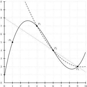
Consider the pointsP0= (1,5), P1= (4,7), P2= (6,4), P3= (9,2). The divided differences are:
x0= 1 [y0] = 5
[y1, y0] = 2 3
x1= 4 [y1] = 7 [y2, y1, y0] =−13
30 [y2, y1] =−3
2 [y3, y2, y1, y0] = 3 40 x2= 6 [y2] = 4 [y3, y2, y1] = 1
6 [y3, y2] =−2
3 x3= 9 [y3] = 2
The corresponding interpolating polynomial are: – when considering pointsP2 andP3:
N23(x) = 2−2/3(x−9) – when considering pointsP1, P2 andP3:
N13(x) = 2−2/3(x−9) + 1/6(x−9)(x−6) – when considering pointsP0, P1, P2 andP3:
N3
0(x) = 2−2/3(x−9) + 1/6(x−9)(x−6) + 3/40(x−9)(x−6)(x−4) These polynomial are presented in Figure1.
4.4 When data points are equidistributed
We consider equidistributed points. More precisely, there existsh >0 such that xi−xi−1=hfori=a+ 1, . . . , b. In this case the interpolating polynomial has a simpler expression.
0 1 2 3 4 5 6 7 8 9 10 0
1 2 3 4 5 6 7 8 9 10
b
P0
bP1
bP2
b
P3
Fig. 1. Interpolating polynomials N23 (dotted), N13 (dashed) and N03 (solid) for the pointsP0= (1,5), P1= (4,7), P2= (6,4), P3= (9,2)
Definition 3. Let (un)n∈N be a numerical sequence. The following notations are defined recursively:
– ∆0(u
n) :=un forn∈N.
– ∆i(u
n) :=∆i−1(un)−∆i−1(un−1)fori∈N∗, n≥i.
Remark that in the literature the notation∇is sometimes used for these differ-ences as they are defined backward.
Using these differences the following lemma allows to simplify the divided differences:
Lemma 1. With the previous notations and considering the data points equidis-tributed, fork=a, . . . , bandi= 0, . . . , k−a:
[yk, . . . , yk−i] =
∆i(y k)
hii!
Proof : Leta≤k≤b. The relation is proven recursively oni.
– Suppose the relation verified fori < k−a. Then:
[yk, . . . , yk
−(i+1)] =
[yk, . . . , yk
−i]−[yk−1, . . . , yk−(i+1)]
xk−xk
−(i+1)
rec. =
∆i(yk) hi
i! − ∆i(yk
−1)
hi i! h(i+ 1) =
∆i
(yk)−∆ i
(yk
−1)
hi+1 (i+ 1)!
def.∆
= ∆
i+1(y k) hi+1
(i+ 1)!
As a consequence the interpolating polynomial has a simpler expression: Proposition 2 (Newton Backward Divided Difference Formula). Using the previous notations and considering the data points equidistributed, the inter-polating polynomial Nb
a evaluated at the pointxb+shwiths∈Ris:
Nb
a(xb+sh) = b−a
X
i=0
s(s+ 1). . .(s+i−1)
i! ∆
i(y b)
Finally the following corollary stands:
Corollary 1. With the previous notations and considering the data points equidis-tributed, the interpolating polynomial Nb
a evaluated at the pointxb+his:
Nab(xb+h) = b−a
X
i=0 ∆i(yb)
4.5 Interpolation error
Interpolation theory leads to consider the following question: if the known data points are constructed using a given function f, i.e.yi =f(xi) fori=a, . . . , b,
how good is approximatedfby the interpolating polynomial? Interpolation error is introduced to answer:
Definition 4. With the previous notations and assuming the existence of a func-tionf such that f(xi) =yi fori=a, . . . , b, the interpolation error is defined as
the distance between the evaluation of the function f and the evaluation of the interpolating polynomial. More precisely forxin the domain off:
eb a(x) :=
¯
¯f(x)−Nab(x)¯¯
5
Link between the Linux entropy estimator and
interpolation polynomial
5.1 Discussion on entropy
Informally the entropy can be interpreted as the unpredictability (random-ness) of a sequence. Even if this don’t rely to the formal definition of entropy, this idea may be an acceptable simplification.
The unpredictability of a sequence can be evaluated by answering the follow-ing question: given a finite set of data, is it possible to guess the next value? This question leads to consider interpolation as a solution. This idea is implemented in the Linux entropy estimator.
5.2 The link
As presented in Section 3.2the Linux entropy estimator computes the amount of entropy of an event as a function of its timing. We consider each event and its timing as a couple (n, tn). Then an estimation of entropy can be computed
con-sidering the interpolation error: when a new event (n, tn) occurs, does it agree
with the pattern of previous values? In other words, how large isen−1
n−1−i(n) for
various value of i? Let evaluate these values. As the data points are equidis-tributed, we have using Corollary1:
en−1
n−1−i(xn) =|yn−Nn
−1
n−1−i(xn−1+h)| =¯¯
¯ yn
|{z}
∆0
(yn)
−∆0(yn−1)
| {z }
∆1(yn)
−∆1(yn−1)
| {z }
∆2(yn)
−. . .
| {z }
...
−∆i(y n−1)
¯ ¯ ¯
=|∆i+1(y
n)|
Using this relation the variableM INn = min(|δ1n|,|δn2|,|δn3|) defined in
Sec-tion3.2can be interpreted as M INn = min
¡
|∆1(tn)|,|∆2(tn)|,|∆3(tn)|
¢
= min¡en−1
n−1(n), en −1
n−2(n), en −1
n−2(n)
¢
In other words the Linux entropy estimator evaluates the entropy of an event by this process:
– Consider the three interpolating polynomials based upon the last three events. – Compute the three interpolation errors according to the new event.
– Take the minimum of these errors.
– Compute the logarithm in base 2 of this minimum (bounded by 0 and 11).
6
Conclusion
Moreover the underlying idea seems to be based upon Kolmogorov complexity rather Shannon entropy. This choice was driven by the constraint that the es-timator as to perform on-the-fly, and then it can not use statistical analysis of the source. Furtherwork may be done on the optimal number of points for the best interpolation (avoiding Runge’s phenomenon).
Acknowledgements
The author would like to thank Marion Videau and Andrea Roeck for their comments.
References
1. Linux kernel,http://kernel.org 1,1,3.1
2. Gutterman, Z., Pinkas, B., Reinman, T.: Analysis of the linux random number generator. IACR Cryptology ePrint Archive 2006, 86 (2006) 1,1,3.2
3. Kolmogorov, A.: Logical basis for information theory and probability theory. Infor-mation Theory, IEEE Transactions on 14(5), 662–664 (1968) 2.1
4. Kolmogorov, A.: Three approaches to the quantitative definition ofinformation’. Problems of information transmission 1, 1–7 (1965) 2.1
5. Lacharme, P., R¨ock, A., Strubel, V., Videau, M.: The linux pseudorandom number generator revisited. IACR Cryptology ePrint Archive 2012, 251 (2012) 1,1,3.2
6. Menezes, A., van Oorschot, P.C., Vanstone, S.A.: Handbook of Applied Cryptogra-phy. CRC Press (1996) 1