DANIEL J. BERNSTEIN AND TANJA LANGE
Abstract. Pollard’s rho algorithm, along with parallelized, vectorized, and negating variants, is the standard method to compute discrete logarithms in generic prime-order groups. This paper presents two reasons that Pollard’s rho algorithm is farther from optimality than generally believed. First, “higher-degree local anti-collisions” make the rho walk less random than the predictions made by the conventional Brent–Pollard heuristic. Second, even a truly ran-dom walk is suboptimal, because it suffers from “global anti-collisions” that can at least partially be avoided. For example, after (1.5 +o(1))√`additions in a group of order`(without fast negation), the baby-step-giant-step method has probability 0.5625 +o(1) of finding a uniform random discrete logarithm; a truly random walk would have probability 0.6753. . .+o(1); and this paper’s new two-grumpy-giants-and-a-baby method has probability 0.71875 +o(1).
1. Introduction
Fix a prime `. The discrete-logarithm problem for a group Gof order ` is the problem of finding loggh, given a generator g of G and an element h of G. The notation logghmeans the unique s ∈ Z/` such that h = gs, where Gis written
multiplicatively.
The difficulty of finding discrete logarithms depends onG. For example, ifGis the additive groupZ/`(encoded as bit strings representing{0,1, . . . , `−1} in the usual way), then logghis simplyh/g, which can be computed in polynomial time
using the extended Euclidean algorithm. As a more difficult example, consider the case thatp= 2`+ 1 is prime and Gis the order-` subgroup of the multiplicative groupF∗p (again encoded in the usual way); index-calculus attacks then run in time subexponential in p and thus in `. However, if G is the order-` subgroup of F∗p
where p−1 is a much larger multiple of `, then index-calculus attacks become much slower in terms of`; the standard algorithms are then the baby-step-giant-step method, using at most (2 +o(1))√`multiplications inG, and the rho method, which if tweaked carefully uses on average (pπ/2 +o(1))√`multiplications in G.
This paper focuses on generic discrete-logarithm algorithms such as the baby-step-giant-step method and the rho method. “Generic” means that these algorithms work for any order-` group G, using oracles to compute 1 ∈ G and to compute a, b7→ab for anya, b∈G. See Section 2 for a precise definition.
If G is an elliptic-curve group chosen according to standard criteria then the best discrete-logarithm algorithms available are variants of the baby-step-giant-step method and the rho method, taking advantage of the negligible cost of computing
Date: 2012.07.09. Permanent ID of this document: 3f5730b1d17389fa4442a4ee5480f668. 2010Mathematics Subject Classification. Primary 11Y16.
This work was supported by the National Science Foundation under grants 0716498 and 1018836 and by the European Commission under Contract ICT-2007-216676 ECRYPT II. No babies (or giants) were harmed in the preparation of this paper.
inverses inG. There is a standard “inverting” (or “negating”) variant of the concept of a generic algorithm, also discussed in Section 2. This paper emphasizes the non-inverting case, but all of the ideas can be adapted to the non-inverting case.
Measuring algorithm cost. The most fundamental metric for generic discrete-logarithm algorithms, and the metric used throughout this paper, is the probability of discovering a uniform random discrete logarithm withinm multiplications. By appropriate integration over mone obtains the average number of multiplications to find a discrete logarithm, the variance, etc. We caution the reader that com-paring probabilities of two algorithms for onemcan produce different results from comparing averages, maxima, etc.; for example, the rho method is faster than baby-step-giant-step on average but much slower in the worst case.
One can interpret a uniform random discrete logarithm as logghfor a uniform random pair (g, h), or as logghfor a fixed gand a uniform random h. The follow-ing trivial “worst-case-to-average-case reduction” shows that a worst-case discrete logarithm is at most negligibly harder than a uniform random discrete logarithm: one computes logghas loggh0−r whereh0 =hgrfor a uniform random r∈Z/`.
There are many reasons that simply counting multiplications, the number m above, does not adequately capture the cost of these algorithms:
• A multiplication count ignores overhead, i.e., costs of computations other than multiplications. For example, the ongoing ECC2K-130 computation uses a very restricted set of Frobenius powers, sacrificing approximately 2% in the number of multiplications, because this reduces the overhead enough to speed up the entire computation.
• A multiplication count ignores issues of memory usage. For some algo-rithms, such as the baby-step-giant-step method, the memory usage grows with √`, while others, such as the rho method, use constant (or near-constant) memory.
• A multiplication count is blind to optimizations of the multiplication oper-ation. The question here is not simply how fast multiplication can be, but how multiplication algorithms interact with higher-level choices in these al-gorithms. For example, Cheon, Hong, and Kim in [10] showed how to look ahead one step in the rho method forF∗p and combine two multiplications
into one with very little overhead, although memory usage increases.
• A multiplication count ignores issues of parallelization. Pollard’s original rho method is difficult to parallelize effectively, but “distinguished point” variants of the rho method are heavily parallelizable with small overhead.
• A multiplication count ignores issues of vectorization. Modern processors can operate on a vector of words in one clock cycle but this requires that the operation is the same across the entire vector. This issue was raised in a recent discussion of whether the negation map on an elliptic curve can actually be used to speed up the rho method, rather than merely to save multiplications; see [6] and [3] for the two sides of the argument.
Contents of this paper. Brent and Pollard in [7] identified a source of non-randomness in the rho method, and quantified the loss of success probability pro-duced by this nonrandomness, under plausible heuristic assumptions. The Brent– Pollard nonrandomness (with various simplifications and in various special cases) has been stated by many authors as the main deficiency in the rho method, and the rho method has been the workhorse of large-scale discrete-logarithm computa-tions. There appears to be a widespread belief that, except for the Brent–Pollard nonrandomness, the rho method is the best conceivable generic discrete-logarithm algorithm. Of course, the rho method can take more than 2√` multiplications in the worst case while the baby-step-giant-step method is guaranteed to finish within 2√`multiplications, but the rho method is believed to be the best way to spend a smaller number of multiplications.
This paper shows that there are actually at least two more steps separating the rho method from optimality. First, the rho method is actually less random and less successful than the Brent–Pollard prediction, because the rho method suffers from a tower of what we call “local anti-collisions”; Brent and Pollard account only for “degree-1 local anti-collisions”. Second, and more importantly, the rho method would not be optimal even if it were perfectly random, because it continues to suffer from what we call “global anti-collisions”. We introduce a new “two grumpy giants and a baby” algorithm that avoids many of these global anti-collisions.
This new algorithm, like the original baby-step-giant-step algorithm, has low overhead but high memory. We have not found a low-memory variant. This means that, for the moment, the algorithm is useful only for discrete-logarithm problems small enough to fit into fast memory. The algorithm nevertheless challenges the idea that the rho method is optimal for larger problems. The same approach might also be useful for “implicit” discrete-logarithm problems in which rho-type iteration is inapplicable, such as stage 2 of thep−1 factorization method, but those problems involve many overheads not considered in this paper.
Section 2 describes the general concept of anti-collisions. Section 3 reviews the Brent–Pollard nonrandomness. Section 4 discusses higher-degree anti-collisions in the rho method. Section 5 reports computations of optimal discrete-logarithm algorithms for small`. Section 6 presents our new algorithm.
We thank the anonymous referees for several useful comments and questions.
2. Anti-collisions
This section introduces the concept of anti-collisions in generic discrete-logarithm algorithms. This section begins by reviewing the standard way to define such algo-rithms; readers familiar with the definition should still skim it to see our notation.
Generic discrete-logarithm algorithms. The standard way to formalize the idea that a generic algorithm works for any order-`groupGis to give the algorithm access to an oracle that computes 1∈Gand an oracle that computes the function a, b 7→ab from G×G to G. The elements of Gare encoded as a size-` set G of strings.
Anm-multiplication generic algorithm is one that calls the a, b7→ab oracle m times. The algorithm obtains 1 for free, and hasg and h as inputs, so overall it seesm+ 3 group elements. We writew0= 1,w1=g, w2 =h, and wi fori≥3 as
the (i−2)nd output of thea, b7→ab oracle: in other words, wi =wjwk for some
These functions can also flip coins (i.e., take as an additional input a sequence b0, b1, . . . of uniform random bits that are independent of each other, of g, of h, etc.), but cannot make oracle calls.
The standard way to formalize the idea that a generic algorithm does not take advantage of the structure of G is to hide this structure by randomizing it. For example, one can takeGas the additive groupZ/`, and takeGas the usual binary representation of {0,1, . . . , `−1}, but choose a uniform random injection fromG to Grather than the usual encoding. One defines the generic success probability of a generic algorithm by averaging not only over logghbut also over the choices
of this injection.
To allow inverting algorithms one also allows free access to an oracle that com-putes a 7→ 1/a. Equivalently, one allows the algorithm to compute wi as either
wjwk or wj/wk, and one also provides 1/wi. Of course, one can simulate this
inversion oracle using approximately lg` calls to the multiplication oracle, since 1/a=a`−1; an algorithm that uses only a small number of inversions can thus be simulated at negligible cost without inversions.
Slopes. Each wi can be written as hxigyi for a pair (xi, yi) ∈ (Z/`)2 trivially
computable by the algorithm. Specifically,w0= 1 =hx0gy0 where (x0, y0) = (0,0); w1=g=hx1gy1 where (x1, y1) = (0,1);w2=h=hx2gy2 where (x2, y2) = (1,0); if wi is computed aswjwk thenwi=hxigyi where (xi, yi) = (xj, yj) + (xk, yk); and
if an inverting algorithm computeswi as wj/wk thenwi=hxigyi where (xi, yi) =
(xj, yj)−(xk, yk).
Normally these algorithms find logghby finding collisions in the map (x, y)7→
hxgy from (Z/`)2 to G. A collision hxigyi =hxjgyj with (x
i, yi)6= (xj, yj) must
have xi 6=xj (otherwisegyi =gyj soyi =yj sinceg generatesG), so the negative
of the slope (yj−yi)/(xj −xi) is exactly loggh. The discrete logarithms found
byw0, w1, . . . , wm+2are thus exactly the negatives of the (m+ 3)(m+ 2)/2 slopes (excluding any infinite slopes) between them+ 3 points (x0, y0), . . . ,(xm+2, ym+2) in (Z/`)2. The number of discrete logarithms found in this way is the numberdof distinct non-infinite slopes. The generic chance of encountering such a collision is exactlyd/`.
In the remaining cases, occurring with probability 1−d/`, these algorithms simply guess loggh. The success chance of this guess is 0 if the guess matches one of the negated slopes discussed above; otherwise the conditional success chance of this guess is 1/(`−d), so the success chance of this guess is 1/`. The overall generic success chance of the algorithm is thus betweend/` and (d+ 1)/`, depending on the strategy for this final guess. In the extreme cased=`this guess does not exist and the generic success chance is 1.
(Similar comments apply to inverting algorithms, but the bound on d is dou-bled, because there are twice as many opportunities to find−loggh. Specifically, comparingwj towifinds the slope (yj−yi)/(xj−xi), while comparingwj to 1/wi
finds (yj+yi)/(xj+xi).)
one measures algorithm cost as the number of multiplications, but is more restric-tive than Shoup’s model in more sophisticated cost metrics; for example, Nechaev’s model is unable to express the rho algorithm.
Chateauneuf, Ling, and Stinson in [9] introduced the idea of counting distinct slopes. They pointed out that the success probability of the baby-step-giant-step method is a factor 2 +o(1) away from the obvious quantification of the Nechaev– Shoup bound: mmultiplications allow only m/2 baby steps and m/2 giant steps, producing m2/4 slopes (all distinct if m2/4 ≤ `), while one can imagine m+ 3 points in (Z/`)2potentially having as many as (m+ 3)(m+ 2)/2> m2/2 distinct slopes.
Computer searches reported in [9, Section 3] found for each ` < 100 a set of only marginally more than √2` points with slopes covering Z/`. However, these sets of points do not form addition chains, and as far as we can tell the shortest addition chains for all of the constructions in [9] are worse than the baby-step-giant-step method in the number of multiplications used. The cost model used in [9] allowsa, b7→asbt as a single oracle call for any (s, t); we view that cost model
as excessively simplified, and are skeptical that algorithms optimized for that cost model will be of any use in practice.
Anti-collisions. We use the word “anti-collision” to refer to an appearance of a useless slope — a slope that cannot create a new collision because the same slope has appeared before. Formally, an anti-collision is a pair (i, j) withi > j such that either
• xi=xj or
• (yj−yi)/(xj−xi) equals (yj0−yi0)/(xj0−xi0) for some pair (i0, j0) lexico-graphically smaller than (i, j) withi0> j0.
The number of anti-collisions is exactly the gap (m+ 3)(m+ 2)/2−d, where as abovedis the number of distinct non-infinite slopes. Our objective in this paper is to understandwhy anti-collisions occur in addition chains in (Z/`)2, and how these anti-collisions can be avoided.
In Section 3 we review a standard heuristic by Brent and Pollard that can be viewed as identifying some anti-collisions in the rho method, making the rho method somewhat less effective than a truly random walk would be. In Section 4 we identify a larger set of anti-collisions in the rho method, making the rho method even less effective than predicted by Brent and Pollard. This difference is most noticeable for rho walks that use a very small number of steps, such as hardware-optimized walks or typical walks on equivalence classes modulo Frobenius on Koblitz curves. It should be obvious that even a truly random walk produces a large number of anti-collisions when m grows to the scale of√`. In Section 6 we show that at least a constant fraction of these anti-collisions can be eliminated: we construct an explicit and efficient addition chain with significantly fewer anti-collisions, and thus significantly higher success probability, than a truly random walk.
3. Review of the Brent–Pollard nonrandomness
discussed in Section 4, these heuristics account for “degree-1 local anti-collisions” but do not account for “higher-degree local anti-collisions”.
The rho method. The rho method precomputesrdistinct “steps”s1, s2, . . . , sr∈
G− {1} (as some initialw’s), and then moves fromwi to wi+1=wisj, wherej is
a function ofwi. Writepj for the probability that stepsj is used.
We suppress standard details of efficient parallelization and collision detection here, since our emphasis is on the success probability achieved after m multipli-cations. Inserting each new group element into an appropriate data structure will immediately recognize the first collision without consuming any multiplications.
The √V formula. Brent and Pollard in [7, Section 2] introduced the following heuristic argument, concluding that if the valuesw0, . . . , wmare distinct thenwm+1 collides with one of those values with probability approximatelymV /`, whereV is defined below. This implies that the total chance of a collision withinm multiplica-tions (i.e., withinw0, . . . , wm+2) is approximately 1−(1−V /`)m
2/2
, which in turn implies that the average number of multiplications for a collision is approximately p
π/2√`/√V. For comparison, a truly random walk would haveV = 1.
This argument applies to a more general form of the rho method, in which some functionF is applied to wi to producewi+1. The first collision might be unlucky enough to involve w0, but otherwise it has the form wi+1 = wj+1 with wi 6=wj,
revealing a collisionF(wi) =F(wj) in the function F. Applications vary in how
they constructF and in the use that they make of a collision.
Assume, heuristically, that the probability ofwimatching any particular valuey
is proportional to the number of preimages ofy, i.e., that Pr[wi=y] = #F−1(y)/`
whereF−1(y) means {x:F(x) =y}. This heuristic is obviously wrong forw 0, but this is a minor error in context; the heuristic seems plausible forw1, . . . , wm, which
are each generated as outputs ofF.
Assume that w0, . . . , wm are distinct. Define X as the set of preimages of
w1, . . . , wm, i.e., the disjoint union ofF−1(w1), . . . , F−1(wm). Then the expected
size ofX is X
x
Pr[x∈X] =X
x
X
i
Pr[F(x) =wi] =
X x X i X y
Pr[F(x) =yandwi=y].
Assume, heuristically, thatF(x) =yandwi=y are independent events. Then the
expected size ofX isP
i
P
y
P
xPr[F(x) =y] Pr[wi=y] =
P
i
P
y#F
−1(y)2/`=
mP
y#F
−1(y)2/`.
Define V as the variance over y of #F−1(y). The average overy of #F−1(y) is 1, so V = (P
y#F
−1(y)2/`)−1, so the expected size of X is mV +m. There
aremknown elementsw0, . . . , wm−1of X; the expected number of elements ofX other thanw0, . . . , wm−1 ismV. By hypothesiswmis none ofw0, . . . , wm−1; ifwm
were uniformly distributed subject to this constraint then it would have probability mV /(`−m)≈mV /`of being inX and thus leading to a collision in the next step.
Thep1−P ip
2
i formula. As part of [1] we introduced the following streamlined heuristic argument, concluding that the collision probability for wm+1 is approxi-mately m(1−P
ip
2
i)/`. This implies that the average number of multiplications
for a collision is approximatelypπ/2√`/p 1−P
ip
2
i.
Fix a group element v, and letw and w0 be two independent uniform random
event occurs if there are distinct i, j such that the following three conditions hold simultaneously:
• v=siw=sjw0; • si is chosen forw; • sj is chosen forw0.
These conditions have probability 1/`2, pi, andpj respectively. Summing over all
(i, j) gives the overall probability P
i6=jpipj
/`2 = P
i,jpipj−Pip
2
i
/`2 =
1−P
ip
2
i
/`2. This means that the probability of an immediate collision fromw andw0 is 1−P
ip2i
/`, where we added over the `choices ofv.
After m+ 3 group elements one has approximately m2/2 potentially colliding pairs. If the inputs to the iteration function were independent uniformly distributed
random points then the probability of success would be 1− 1− 1−P
ip
2
i
/`m2/2 and the average number of iterations before a collision would be approximately p
π/2√`/p1−P
ip2i. The inputs to the iteration function in Pollard’s rho method
are not actually independent, but this has no obvious effect on the average number of iterations.
Relating the two formulas. We originally obtained the formulap1−P
ip
2
i by
specializing and simplifying the Brent–Pollard√V formula as follows.
The potential preimages ofyarey/s1, y/s2, . . . , y/sr, which are actual preimages
with probabilities p1, p2, . . . , pr respectively. A subset I of {1,2, . . . , r} matches
the set of indices of preimages with probability (Q
i∈Spi)(Qi /∈S(1−pi)), so the
average of #F−1(y)2isP
I#I
2(Q
i∈Spi)(Qi /∈S(1−pi)). It is easy to see that most
monomials (e.g., p1p2p3) have coefficient 0 in this sum; the only exceptions are linear monomialspi, which have coefficient 1, and quadratic monomialspipj with
i < j, which have coefficient 2. The sum therefore equalsP
ipi+ 2
P
i,j:i<jpipj=
P
ipi+ (Pipi)2−Pip
2
i = 2−
P
ip
2
i. HenceV = 1−
P
ip
2
i.
The p1−1/r formula. In traditional “adding walks” (credited to Lenstra in [20, page 66]; see also [21, page 295] and [25]), each pi is 1/r, and
p 1−P
ip
2
i
is p1−1/r. This p1−1/r formula first appeared in [25], with credit to the subsequent paper [4] by Blackburn and Murphy. The heuristic argument in [4] is the same as the Brent–Pollard argument.
Case study: Koblitz curves. Thep1−P
ip
2
i formula was first used to optimize
walks on Koblitz curves. These walks map a curve pointW toW+ϕi(W), where ϕ is the Frobenius map and i is chosen as a function of the Hamming weight of the normal-basis representation of thex-coordinate ofW. The Hamming weight is not uniformly distributed, and any reasonable function of the Hamming weight is also not uniformly distributed, so thep1−1/rformula does not apply. Note that these are “multiplying walks” rather than “adding walks” (ifW =xiH+yiGthen
W +ϕi(W) =sixiH+siyiGfor certain constantssi∈(Z/`)∗), but the heuristics
in this section are trivially adapted to this setting.
time of 1/ q
1−P
i
131 2i
2
/2260 ≈ 1.053211, even if all 66 weights use different scalars si. We extract just 3 bits of weight information, using only 8 different
values for the scalars, to reduce the time per iteration. The values are determined by HW(xPi)/2 mod 8; the distribution of
P
i
131 16i+2j
for 0≤j ≤7 gives probabilities
0.1414,0.1443,0.1359,0.1212,0.1086,0.1057,0.1141,0.1288,
giving a total increase of the number of iterations by a factor of 1.069993.
4. Higher-degree local anti-collisions
Consider the rho method using r “steps” s1, s2, . . . , sr ∈ G, as in the previous
section. The method multiplieswi by one of these steps to obtainwi+1, multiplies wi+1 by one of these steps to obtainwi+2, etc.
Assume that the step wi+1/wi is different from the step wi+2/wi+1, but that wi+1/wi is the same as an earlier stepwj+2/wj+1, and thatwi+2/wi+1 is the same as the stepwj+1/wj. There are anti-collisions (i+ 1, j+ 2) and (i+ 2, j+ 1), exactly
the phenomenon discussed in the previous section: for example,wi+1 cannot equal wj+2unlesswiequalswj+1. There is, however, also a local anti-collision (i+2, j+2) not discussed in the previous section: wi+2cannot equalwj+2 unlesswi equalswj.
The point is that the ratiowi+2/wiis a product of two steps, and the ratiowi+2/wi
is a product of the same two steps in the opposite order.
We compute the heuristic impact of these “degree-2 local anti-collisions”, to-gether with the degree-1 local anti-collisions of Section 3, as follows. Assume for simplicity that 1, s1, s2, . . . , sr, s21, s1s2, . . . , s1sr, s22, . . . , s2sr, . . . , s2r−1, sr−1sr, s2r
are distinct. WriteF(w) for the group element thatwmaps to. Fix a group element v, and consider the event that two independent uniform random group elements w, w0 have F(F(w)) =v=F(F(w0)) with no collisions among w, w0, F(w), F(w0). This event occurs if there arei, i0, j, j0 withsj6=sj0 andsjsi6=sj0si0 such that the following conditions hold simultaneously:
• v=sjsiw=sj0si0w0;
• F(w) =siw; • F(siw) =sjsiw; • F(w0) =si0w0;
• F(si0w0) =sj0si0w0.
These conditions have probability 1/`2, pi, pj, pi0, and pj0 respectively. Given the first condition, the remaining conditions are independent of each other, since w = v/(sjsi), siw = v/sj, w0 = v/(sj0si0), and si0w0 = v/sj0 are distinct. This event thus has probability P
pipjpi0pj0/`2 where the sum is over all i, j, i0, j0 with sj 6= sj0 and sjsi =6 sj0si0. The complement of the sum is over all i, j, i0, j0 with sj =sj0 or sjsi =sj0si0, i.e., withj =j0 or withi0 =j6=j0 =i. The complement is thusP
jp
2
j+
P
i,j:i6=jp
2
ip2j =
P
jp
2
j+ (
P
jp
2
j)2−
P
jp
4
j, and the original sum is
1−P
jp
2
j −(
P
jp
2
j)
2+P
jp
4
j. Adding over allv gives probability (1−
P jp 2 j− (P jp 2 j)
2+P
jp
4
j)/`of this type of two-step collision betweenwand w0.
For example, ifpi= 1/rfor alli, then the degree-1-and-2 nonrandomness factor
Beyond degree 2. More generally, a “degree-klocal anti-collision” (i+k, j+k) occurs when the product of k successive steps wi+1/wi, wi+2/wi+1, etc. matches the product ofksuccessive stepswj+1/wj,wj+2/wj+1, etc., without a lower-degree local anti-collision occurring. A “degree-(k, k0) local anti-collision” (i+k, j+k0) is
defined similarly.
Given the vector (s1, s2, . . . , sr), one can straightforwardly compute the overall
heuristic effect of local anti-collisions of degree at mostk, by summing the products pi1· · ·pikpi01· · ·pi0k for which 1,si1,si
0
1,si1si2,si01si02, etc. are distinct. Experiments indicate that the largest contribution is usually from the smallest degrees.
We emphasize that the results depend on the vector (s1, s2, . . . , sr), because
generic commutative-group equations such ass1s2 =s2s1 are not the only multi-plicative dependencies amongs1, s2, . . . , sr. One can check that s1, s2, . . . , sr have
no non-generic multiplicative dependencies of small degree (and modify them to avoid such dependencies), but they always have medium-degree non-generic mul-tiplicative dependencies, including mixed-degree non-generic mulmul-tiplicative depen-dencies.
Ifs1, s2, . . . , srhave only generic dependencies of degree at mostkthen the sum
described above is expressible as a polynomial in the easily computed quantities X2 = Pjp
2
j, X4 = Pjp
4
j, etc., by a simple inclusion-exclusion argument. For
example, the degree-1 nonrandomness factor is 1/√1−X2, as in Section 3; the degree-≤2 nonrandomness factor is 1/p1−X2−X22+X4, as explained above; the degree-≤3 nonrandomness factor is 1/p1−X2−X22+X4−3X23+ 7X2X4−4X6; the degree-≤4 nonrandomness factor is
1/p1−X2−X22+X4−3X23+7X2X4−4X6−13X24+53X22X4−56X2X6−17X42+33X8;
etc. In the uniform case these factors are 1/p1−1/r, 1/p1−1/r−1/r2+ 1/r3, 1/p1−1/r−1/r2−2/r3+ 7/r4−4/r5, etc.
Case study: r = 6. Hildebrand showed in [13] that almost everyr-adding walk (with pj = 1/r) reaches a nearly uniform distribution in Z/` within O(`2/(r−1))
steps; in particular, withino(√`) steps forr≥6. Implementors optimizing Pollard’s rho method for hardware often want rto be as small as possible (to minimize the storage required for precomputed steps and the cost of accessing that storage), and in light of Hildebrand’s result can reasonably chooser= 6. This raises the question of how random a 6-adding walk is; perhaps it is better to take a larger value of r, increasing overhead but reducing nonrandomness.
Forr= 6, withp1=p2 =p3=p4 =p5 =p6= 1/6 and generic s1, . . . , s6, the heuristic nonrandomness factors are approximately 1.095445 for degree 1; 1.110984 for degree ≤ 2; 1.117208 for degree ≤ 3; 1.120473 for degree ≤ 4; 1.122452 for degree≤5; 1.123767 for degree≤6; 1.124696 for degree≤7; 1.125383 for degree
≤8; 1.125909 for degree≤9; 1.126322 for degree≤10; 1.126654 for degree≤11; 1.126926 for degree ≤ 12; 1.127151 for degree ≤ 13; 1.127341 for degree ≤ 14; 1.127503 for degree≤ 15; etc. These factors converge to 1.129162 as the degree increases; see Appendix A. Evidently the Brent–Pollard heuristic capturesmost of the impact of local anti-collisions forr= 6, but not all of the impact.
` factor experiments
1009 1.150103 230
10007 1.147846 230 100003 1.141268 230 1000003 1.136129 230 10000019 1.132923 230 100000007 1.131149 229 1000000007 1.130136 227 10000000019 1.129580 224
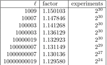
Table 4.1. Observed average walk length until a collision, for a uniform random walk in Z/` using 6 uniform random steps. “Factor” is the observed average walk length divided bypπ/2√`, rounded to 6 digits after the decimal point. “Experiments” is the number of experiments carried out for`.
using s1, s2, . . . , s6 with equal probability, and stopped at the first collision. The average walk length was approximately 1.150103 timespπ/2√`; note that this does not count the multiplications used to generates1, s2, . . . , s6. We then tried several larger values of`; the resulting nonrandomness factors are shown in Table 4.1. Our heuristics predict that these numbers will converge to approximately 1.129162 as `→ ∞, rather than 1.095445.
Note that for small`there is a larger chance of low-degree dependencies among the stepssi, so it is not a surprise that smaller values of`have larger nonrandomness
factors. We do not know whether a quantitative analysis of this phenomenon would predict the numbers shown in Table 4.1 for small `, or whether other phenomena also play a role.
Case study: Koblitz curves, revisited. Consider again the ECC2K-130 walk introduced in [1]. Here`= 680564733841876926932320129493409985129.
For 0 ≤ j ≤ 7 define ϕ as the Frobenius map on the ECC2K-130 curve, and definesj ∈Z/`as 1 + 196511074115861092422032515080945363956j+3. This walk
moves from P to P+ϕj+3(P) =sjP if the Hamming weight of thex-coordinate
of P is congruent to 2j modulo 16; this occurs with probability (almost exactly) pj=Pi 16131i+2j/2130.
The only small-degree multiplicative dependencies amongs0, . . . , s7 are generic commutative-group equations such as s1s2 = s2s1. We already reported this in [1, Section 2] to explain why the walk is highly unlikely to enter a short cycle. We point out here that this has a larger effect, namely minimizing small-degree anti-collisions. We now analyze the impact of the small-degree anti-collisions that remain, those that arise from the generic commutative-group equations.
For degree 1 the nonrandomness factor is 1/√1−X2 ≈ 1.069993. For degree
≤2 the nonrandomness factor is 1/p1−X2−X22+X4 ≈1.078620. For degree
Case study: Mixed walks. The same type of analysis should also apply to “mixed walks” combining non-commuting steps such asw7→ws1, w7→ws2, and w7→w2. However, we have not yet carried out experiments.
Optimizing asymptotics. It is frequently stated that the rho method, like a truly random walk, finishes in (pπ/2 +o(1))√` multiplications on average.
However, the experimental results by Sattler and Schnorr [20, page 76] and by Teske [25] showed clearly thatpπ/2 +o(1) is not achieved by small values ofr, and in particular by Pollard’s original rho method. The Brent–Pollard nonrandomness, and in particular thep1−1/rformula, indicates thatpπ/2 +o(1) is not achieved by any boundedr; one must have 1/r∈o(1), i.e.,r→ ∞as`→ ∞. On the other hand, ifrgrows too quickly then the cost of setting uprsteps is nonnegligible.
This analysis does not contradictpπ/2 +o(1). However, it does indicate that some care is required in the algorithm details, and thatpπ/2+o(1) can be replaced bypπ/2 +O(`−1/4) but not bypπ/2 +o(`−1/4).
To optimize theo(1) one might try choosing steps that are particularly easy to compute. For example, one might takes3 =s1s2,s4 =s2s3, etc., where s1, s2 are random. We point out, however, that such choices are particularly prone to higher-degree anti-collisions. We recommend taking into account not just the number of steps and the number of multiplications required to precompute those steps, but also the impact of higher-degree anti-collisions.
5. Searching for better chains for small primes
If ` is small then by simply enumerating addition chains one can find generic discrete-logarithm algorithms that use fewer multiplications than the rho method. This section reports, for each small prime`, the results of two different computer searches. One search greedily obtained as many slopes as it could after each multi-plication, deferring anti-collisions as long as possible. The other search minimized the number of multiplications required to find an average slope. Chains found by such searches are directly usable in discrete-logarithm computations for these val-ues of`; perhaps they also provide some indication of what one can hope to achieve for much larger values of`. These searches also show that merely counting the size of a slope cover, as in [9, Section 3], underestimates the cost of discrete-logarithm algorithms, although one can hope that the gap becomes negligible as`increases.
A continuing theme in this section is that the obvious quantification of the Nechaev–Shoup bound is not tight. The bound says that anm-addition chain has
≤(m+ 3)(m+ 2)/2 slopes; but there is actually a gap, increasing withm, between (m+ 3)(m+ 2)/2 and the maximum number of slopes in an m-addition chain. This section explains part of this gap by identifying two types of anti-collisions that addition chains cannot avoid and stating an improved bound that accounts for these anti-collisions. However, the improved bound is still not tight for most of these values of`, and for long chains the improved bound is only negligibly stronger than the Nechaev–Shoup bound.
Greedy slopes. Definedias the number of distinct finite slopes among the points
(x0, y0),(x1, y1),(x2, y2), . . . ,(xi, yi) in (Z/`)2. For example, the chain
in (Z/7)2has (d0, d1, d2, d3, d4, d5) = (0,0,2,3,5,7): there are 2 distinct finite slopes among (0,0),(0,1),(1,0); 3 distinct finite slopes among (0,0),(0,1),(1,0),(0,2); 5 distinct finite slopes among (0,0),(0,1),(1,0),(0,2),(1,2); and 7 distinct finite slopes among (0,0),(0,1),(1,0),(0,2),(1,2),(1,4).
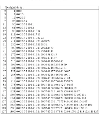
For each prime` <128 we computed the lexicographically maximum sequence (d0, d1, . . .) for all infinite addition chains starting (0,0),(0,1),(1,0) in (Z/`)2. These maxima, truncated to the first occurrence of`, are displayed in Table 5.1. For example, Table 5.1 lists (0,0,2,3,5,7) for`= 7, indicating that the lexicographic maximum is (0,0,2,3,5,7,7,7,7,7, . . .): one always hasd0= 0,d1= 0, andd2= 2; the maximum possibled3 is 3; givend3 = 3, the maximum possibled4 is 5; given d3= 3 andd4= 5, the maximum possibled5 is 7.
This computation was not quite instantaneous, because it naturally ended up computing all finite chains achieving the truncated maximum (and, along the way, all chains achieving every prefix of the truncated maximum). There are, e.g., 5420 length-21 chains that match the (d0, d1, . . .) shown in Table 5.1 for`= 109.
Minimal weight. We also computed`-slope addition chains of minimal weight for each prime` <48. Here “weight” meansP
i≥1i(di−di−1). Dividing this weight by`produces the average, over alls∈Z/`, of the number of multiplications (plus 2 to account for the inputs g and h) used to find slope s. It might make more sense to compute (`−1)-slope addition chains of minimal weight, since a generic discrete-logarithm algorithm that finds `−1 slopes also recognizes the remaining slope by exclusion, but the gap becomes negligible as`increases.
Lexicographically maximizing (d0, d1, . . .), as in Table 5.1, does not always pro-duce minimal-weight`-slope addition chains. For example, the chain
(0,0),(0,1),(1,0),(0,2),(0,3),(1,3),(1,6),(2,12),(2,14),(2,16),(3,17),(4,28)
for ` = 29 has weight 210 with (d0, d1, . . .) = (0,0,2,3,4,7,10,14,19,23,27,29), while chains achieving the lexicographic maximum in Table 5.1 have weight 211. We similarly found weight 299 (compared to 300) for`= 37, weight 372 (compared to 375) for ` = 43, and weight 423 (compared to 425) for` = 47. It is not clear whether this gap becomes negligible as`increases.
Some obstructions. We explain here two simple ways that anti-collisions appear in addition chains. Every addition chain produces at least a linear number of anti-collisions that follow these simple patterns.
First, doubling a point (xj, yj) produces two anti-collisions: the slopes from
2(xj, yj) to (xj, yj) and to (0,0) are the same as the slope from (xj, yj) to (0,0).
Doubling another point (xk, yk) produces three anti-collisions: the slope from
2(xk, yk) to 2(xj, yj) is the same as the slope from (xk, yk) to (xj, yj). A third
doubling produces four anti-collisions, and so on; doubling n points produces a total ofn(n+ 3)/2 anti-collisions of this type.
Second, adding (xi, yi) to a distinct point (xj, yj) produces two anti-collisions:
the slopes from (xi, yi)+(xj, yj) to (xi, yi) and to (xj, yj) are the same as the slopes
from (xj, yj) and from (xi, yi) to (0,0). Subsequently adding the same (xi, yi) to
another point (xk, yk) produces three anti-collisions: the slope from (xi, yi)+(xk, yk)
to (xi, yi) + (xj, yj) is the same as the slope from (xk, yk) to (xj, yj), exactly as in
Section 3.
` weight d0d1 . . . 2 4 0 0 2 3 7 0 0 2 3 5 15 0 0 2 3 5 7 25 0 0 2 3 5 7 11 50 0 0 2 3 5 7 10 11 13 64 0 0 2 3 5 7 10 13 17 96 0 0 2 3 5 7 10 14 16 17 19 113 0 0 2 3 5 7 10 14 17 19 23 148 0 0 2 3 5 7 10 14 19 22 23 29 211 0 0 2 3 5 7 10 14 19 23 26 28 29 31 230 0 0 2 3 5 7 10 14 19 23 28 31 37 300 0 0 2 3 5 7 10 14 19 23 29 33 36 37 41 347 0 0 2 3 5 7 10 14 19 24 29 34 39 41 43 375 0 0 2 3 5 7 10 14 19 24 29 34 38 42 43 47 425 0 0 2 3 5 7 10 14 19 24 30 35 40 44 47 53 510 0 0 2 3 5 7 10 14 19 24 30 36 41 45 50 52 53 59 596 0 0 2 3 5 7 10 14 19 24 30 36 42 48 52 57 58 59 61 631 0 0 2 3 5 7 10 14 19 24 30 35 42 48 52 56 59 61 67 727 0 0 2 3 5 7 10 14 19 24 30 36 41 47 53 59 63 66 67 71 788 0 0 2 3 5 7 10 14 19 24 30 36 42 48 54 60 66 70 71 73 815 0 0 2 3 5 7 10 14 19 24 30 36 43 50 56 62 67 71 73 79 919 0 0 2 3 5 7 10 14 19 24 30 37 43 49 57 64 69 73 76 79 83 978 0 0 2 3 5 7 10 14 19 24 30 37 44 51 59 65 72 77 80 83 89 1081 0 0 2 3 5 7 10 14 19 24 30 37 44 53 60 66 74 80 84 87 89 97 1224 0 0 2 3 5 7 10 14 19 24 30 37 44 51 61 69 78 83 88 92 96 97 101 1307 0 0 2 3 5 7 10 14 19 24 30 37 45 53 60 69 76 82 89 93 97 100 101 103 1351 0 0 2 3 5 7 10 14 19 24 30 37 45 52 60 67 74 83 89 94 98 102 103 107 1422 0 0 2 3 5 7 10 14 19 24 30 37 45 53 61 70 77 84 91 96 100 104 107 109 1466 0 0 2 3 5 7 10 14 19 24 30 37 44 52 60 68 77 84 91 98 102 106 108 109 113 1536 0 0 2 3 5 7 10 14 19 24 30 37 44 52 62 70 78 86 94 99 105 109 113
127 1806 0 0 2 3 5 7 10 14 19 24 30 37 45 53 63 73 84 92 98 105 112 118 122 126 127
Table 5.1. For each ` < 128, the lexicographically maximum (d0, d1, . . .). “Weight” means Pi≥1i(di−di−1).
at least two anti-collisions, and therefore produces at most one new slope to the previous three points; this explains the 3. The second addition also produces at least two anti-collisions, and therefore at most two new slopes to the previous four points; this explains the 5. One might think that the next step is 8, but having only two anti-collisions in each of the first three additions would imply that those three additions include at most one doubling and no other reuse of summands, for a total of at least five summands, while there are only four non-zero summands available for the first three additions.
and thus a total of at most (m+ 3)(m+ 2)/2−(3m−1) = (m2−m+ 8)/2 slopes. This explains 5,7,10,14,19 in Table 5.1 but does not explain 24.
6. Two grumpy giants and a baby
This section presents the algorithm featured in the title of this paper. This algorithm is, as the name suggests, a modification to the standard baby-step-giant-step method. The modification increases the number of different slopes produced withinmmultiplications, and for a typical range ofmincreases the number beyond the effectiveness of the rho method.
In the baby-step-giant-step algorithm the baby steps computehxigyifor (x
i, yi)∈
(0,0) +{0,1,2, . . . ,d√`e}(0,1) and the giant steps compute hxigyi for (x
i, yi) ∈
(1,0) +{0,1,2, . . . ,b√`c}(0,d√`e). The first observation is that the slopes within one type of step are constant; the second observation is that once all steps are done all`slopes appear. Our idea is to make the lines of fixed slope shorter, i.e. introduce more players. Note that introducing a second baby is not useful: lines between the points in (x, y) +{0,1,2, . . . ,d√`e}(0,1) and (0,0) +{0,1,2, . . . ,d√`e}(0,1) repeat each slope≈√`times. We thus need to introduce more giants to make progress.
The two-grumpy-giants-and-a-baby method is parametrized by a positive integer n, normally proportional to√`; the reader should imaginenbeing approximately 0.5√`. The number of multiplications in the method is approximately 3n. Here is the set of points (xi, yi)∈(Z/`)2 produced by the method:
Baby: (0,0) +{0, . . . , n−1}(0,1)
Giant1: (1,0) +{1, . . . , n}(0, n)
Giant2: (2,0)− {1, . . . , n}(0, n+ 1)
The initial negation (0,−(n+ 1)) for Giant2 has negligible cost, approximately lg`multiplications. Choosingnandn+1 for the steps in theydirection for the two giants gives a good coverage of slopes sincenandn+ 1 are coprime. The grumpy giants make big steps (on the scale of√`) and quickly walk in opposite directions away from each other. Luckily they are not minding the baby.
We now analyze the slopes covered by this method. Again it is not interesting to look at the slopes among one type of points. The slope between a point (0, i) in the Baby set and a point (1, jn) in the Giant1 set isjn−i; this means that all slopes in
{1, . . . , n2}are covered. The slope between (0, i) in the Baby set and (2,−j(n+ 1)) in the Giant2 set is (−j(n+ 1)−i)/2∈
−n2−2n+ 1, . . . ,−n−1 /2; there aren2 distinct slopes here, almost exactly covering
−n2−2n+ 1, . . . ,−n−1 /2. The slope between (1, in) in the Giant1 set and (2,−j(n+ 1)) in the Giant2 set is
−j(n+ 1)−in ∈
−2n2−n, . . . ,−2n−1 ; there are another n2 distinct slopes here, covering about half the elements of
−2n2−n, . . . ,−2n−1 .
To summarize, there are three sets ofn2distinct slopes here, all between−2n2− n+ 1 andn2. One can hope for a total of 3n2 distinct slopes if` >3n2+n, but this hope runs into two obstacles. The first obstacle is that the “odd” elements of
−n2−2n+ 1, . . . ,−n−1 can bump into the other sets when computing (2i+ 1)/2 =i+(`+1/2); but for`∈4n2+O(n) this effect loses onlyO(n) elements. The second obstacle is that any Giant1–Giant2 slopes between (−n2−2n)/2 and (−n−
2)/2 will bump into −n2−2n+ 1, . . . ,−n−1 /2 for the the “even” elements of
this interval. Overall there are 23n2/8 +O(n) distinct slopes, i.e., (0.71875 +o(1))` distinct slopes.
For comparison, the same (3 +o(1))n multiplications allow the original baby-step-giant-step method to compute (1.5 +o(1))nbaby steps and (1.5 +o(1))ngiant steps, producing only (2.25 +o(1))n2= (0.5625 +o(1))`distinct slopes. The same number of multiplications in the rho method (with 1/o(1) different steps, simulating a uniform random walk within a factor 1 +o(1)) produces (9 +o(1))n2/2 = (1.125 + o(1))`random slopes, and thus (1−exp(1.125)+o(1))`= (0.6753. . .+o(1))`distinct slopes with overwhelming probability. We have performed computer experiments to check each of these numbers.
Weighing the giants. We repeat a warning from Section 1: one algorithm can be better than another after a particular number of multiplications but nevertheless have worse average-case performance.
For example, the baby-step-giant-step method has two standard variants, which we call the baby-steps-then-giant-steps method (introduced by Shanks in [22, pages 419–420]) and the interleaved-baby-step-giant-step method (introduced much later by Pollard in [17, page 439, top]). Both variants (with giant steps chosen to be of size (1+o(1))√`) reach 100% success probability using (2+o(1))√`multiplications, while the rho method has a lower success probability for that number of multiplica-tions. Average-case performance tells a quite different story: the baby-steps-then-giant-steps method uses (1.5 +o(1))√`multiplications on average; the interleaved-baby-step-giant-step method is better, using (4/3 +o(1))√`= (1.3333. . .+o(1))√` multiplications on average; the rho method is best, using (pπ/2 +o(1))√` = (1.2533. . .+o(1))√`multiplications on average.
Our analysis above shows that the two-grumpy-giants-and-a-baby method is more effective than the rho method (and the baby-step-giant-step method) as a way to use (1.5 +o(1))√` multiplications. One might nevertheless guess that the rho method has better average-case performance; for example, an anonymous referee stated that the new method “presumably has worse average-case running time”.
Our computer experiments indicate that the (interleaved-)two-grumpy-giants-and-a-baby method actually has better average-case running time than the rho method. For example, for ` = 65537, we found a chain of weight 20644183 = (1.23046. . .)`1.5 with the two-grumpy-giants-and-a-baby method. Here we chose n= 146, used (suboptimal) binary addition chains for (0, n) and (0, `−n−1), and then cycled between points (0, i) and (1, in) and (2,−i(n+1)) until we had`different slopes. For`= 1000003 we found a chain of weight 1205458963 = (1.20545. . .)`1.5 in the same way withn= 558.
References
[1] Daniel V. Bailey, Lejla Batina, Daniel J. Bernstein, Peter Birkner, Joppe W. Bos, Hsieh-Chung Chen, Chen-Mou Cheng, Gauthier van Damme, Giacomo de Meulenaer, Luis Ju-lian Dominguez Perez, Junfeng Fan, Tim G¨uneysu, Frank Gurkaynak, Thorsten Kleinjung, Tanja Lange, Nele Mentens, Ruben Niederhagen, Christof Paar, Francesco Regazzoni, Peter Schwabe, Leif Uhsadel, Anthony Van Herrewege, Bo-Yin Yang,Breaking ECC2K-130(2009). URL:http://eprint.iacr.org/2009/541. Citations in this document: §3,§3,§4,§4. [2] Pierre Barrucand, Sur la somme des puissances des coefficients multinomiaux et les
puis-sances successives d’une fonction de Bessel, Comptes Rendus des S´eances de l’Acad´emie des Sciences 258 (1964), 5318–5320. URL:http://gallica.bnf.fr/ark:/12148/cb343481087/ date.r=.langEN. Citations in this document: §A,§A.
[3] Daniel J. Bernstein, Tanja Lange, Peter Schwabe,On the correct use of the negation map in the Pollard rho method, in PKC 2011 [8] (2011), 128–146. URL:http://eprint.iacr.org/ 2011/003. Citations in this document: §1.
[4] Simon R. Blackburn, Sean Murphy,The number of partitions in Pollard rho, technical re-port RHUL-MA-2011-11, Department of Mathematics, Royal Holloway, University of London (2011). URL: http://www.ma.rhul.ac.uk/static/techrep/2011/RHUL-MA-2011-11.pdf. Ci-tations in this document: §3,§3.
[5] Jonathan M. Borwein, Dirk Nuyens, Armin Straub, James Wan, Some arithmetic proper-ties of short random walk integrals, Ramanujan Journal26(2011), 109–132. URL:http:// arminstraub.com/pub/random-walk-integrals. Citations in this document: §A.
[6] Joppe W. Bos, Thorsten Kleinjung, Arjen K. Lenstra,On the use of the negation map in the Pollard rho method, in ANTS 2010 [12] (2010), 66–82. URL:http://infoscience.epfl.ch/ record/164553/files/NPDF-45.pdf. Citations in this document: §1.
[7] Richard P. Brent, John M. Pollard,Factorization of the eighth Fermat number, Mathematics of Computation36(1981), 627–630. ISSN 0025–5718. MR 83h:10014. URL:http://www.cs. ox.ac.uk/people/richard.brent/pub/pub061.html. Citations in this document: §1,§3. [8] Dario Catalano, Nelly Fazio, Rosario Gennaro, Antonio Nicolosi (editors), Public key
cryptography — PKC 2011 — 14th international conference on practice and theory in pub-lic key cryptography, Taormina, Italy, March 6–9, 2011, Lecture Notes in Computer Science, 6571, Springer, 2011. See [3].
[9] M. A. Chateauneuf, Alan C. H. Ling, Douglas R. Stinson,Slope packings and coverings, and generic algorithms for the discrete logarithm problem, Journal of Combinatorial Designs11 (2003), 36–50. URL:http://eprint.iacr.org/2001/094. Citations in this document:§2,§2, §2,§2,§5.
[10] Jung Hee Cheon, Jin Hong, Minkyu Kim, Speeding up the Pollard rho method on prime fields, in Asiacrypt 2008 [16] (2008), 471–488. URL:http://www.iacr.org/archive/ asiacrypt2008/53500477/53500477.pdf. Citations in this document: §1.
[11] Walter Fumy (editor),Advances in cryptology — EUROCRYPT ’97, international conference on the theory and application of cryptographic techniques, Konstanz, Germany, May 11–15, 1997, Lecture Notes in Computer Science, 1233, Springer, 1997. See [24].
[12] Guillaume Hanrot, Fran¸cois Morain, Emmanuel Thom´e (editors),Algorithmic number theory, 9th international symposium, ANTS-IX, Nancy, France, July 19–23, 2010, Lecture Notes in Computer Science, 6197, Springer, 2010. See [6].
[13] Martin Hildebrand,Random walks supported on random points ofZ/nZ, Probability Theory and Related Fields100(1994), 191–203. MR 95j:60015. Citations in this document:§4. [14] Donald J. Lewis (editor),1969 Number Theory Institute: proceedings of the 1969 summer
institute on number theory: analytic number theory, Diophantine problems, and algebraic number theory; held at the State University of New York at Stony Brook, Stony Brook, Long Island, New York, July 7–August 1, 1969, Proceedings of Symposia in Pure Mathematics, 20, American Mathematical Society, Providence, Rhode Island, 1971. ISBN 0-8218-1420-6. MR 47:3286. See [22].
[15] Vasili˘ı I. Nechaev,Complexity of a determinate algorithm for the discrete logarithm, Math-ematical Notes55(1994), 165–172. Citations in this document:§2.
Australia, December 7–11, 2008, Lecture Notes in Computer Science, 5350, Springer, 2008. See [10].
[17] John M. Pollard,Kangaroos, Monopoly and discrete logarithms, Journal of Cryptology13 (2000), 437–447. Citations in this document: §6.
[18] Bruce Richmond, Cecil Rousseau, A multinomial summation: Comment on Problem 87-2, SIAM Review 31 (1989), 122–125. URL: http://epubs.siam.org/sirev/resource/1/ siread/v31/i1. Citations in this document: §A,§A,§A.
[19] L. B. Richmond, Jeffrey Shallit, Counting abelian squares, Electronic Journal of Com-binatorics 16 (2009), Research Paper 72, 9 pp. ISSN 1077-8926. URL: http://www. combinatorics.org/Volume_16/PDF/v16i1r72.pdf. Citations in this document: §A,§A,§A, §A.
[20] J¨urgen Sattler, Claus-Peter Schnorr,Generating random walks in groups, Annales Univer-sitatis Scientiarum Budapestinensis de Rolando E¨otv¨os Nominatae. Sectio Computatorica 6 (1989), 65–79. ISSN 0138-9491. MR 89a:68108. URL:http://ac.inf.elte.hu/Vol_006_ 1985/065.pdf. Citations in this document: §3,§4.
[21] Claus-Peter Schnorr, Hendrik W. Lenstra, Jr., A Monte Carlo factoring algorithm with linear storage, Mathematics of Computation 43 (1984), 289–311. ISSN 0025-5718. MR 85d:11106. URL: http://www.ams.org/mcom/1984-43-167/S0025-5718-1984-0744939-5/ S0025-5718-1984-0744939-5.pdf. Citations in this document: §3.
[22] Daniel Shanks,Class number, a theory of factorization, and genera, in [14] (1971), 415–440. MR 47:4932. Citations in this document: §6.
[23] Neil J. A. Sloane,The on-line encyclopedia of integer sequences(2012). URL:http://oeis. org. Citations in this document: §A.
[24] Victor Shoup,Lower bounds for discrete logarithms and related problems, in EUROCRYPT 1997 [11] (1997), 256–266. URL:http://www.shoup.net/papers/. Citations in this document: §2.
[25] Edlyn Teske, On random walks for Pollard’s rho method, Mathematics of Com-putation 70 (2001), 809–825. URL: http://www.ams.org/journals/mcom/2001-70-234/ S0025-5718-00-01213-8/S0025-5718-00-01213-8.pdf. Citations in this document: §3,§3, §4.
Appendix A. Computing limits of anti-collision factors
This appendix shows, for each integer r >3, a reasonably fast method to com-pute the limit of the sequence of generic uniform heuristic nonrandomness factors 1/p1−1/r, 1/p1−1/r−1/r2+ 1/r3, 1/p
1−1/r−1/r2−2/r3+ 7/r4−4/r5, etc. considered in Section 4. For example, these factors converge to approximately 1.129162 forr= 6.
We are indebted to Neil Sloane’s Online Encyclopedia of Integer Sequences [23] for leading us to [5] (by a search for the integer 4229523740916 shown below), and to Armin Straub for explaining how to use [2] and [18] to compute the sumP
kuk/r2k
discussed here. Our contribution here is the connection described below between anti-collision factors and sums of squares of multinomials.
Review of sums of squares of multinomials. DefineU =P
i
P
jsi/sj in the
r-variable function field Q(s1, . . . , sr), and define uk as the constant coefficient of
Uk. Consider the problem of computingP
k≥0uk/r2k.
Note that Uk = P
i1,...,ik
P
j1,...,jksi1· · ·sik/sj1· · ·sjk, so uk is the number
of tuples (i1, . . . , ik, j1, . . . , jk) such that si1· · ·sik/sj1· · ·sjk = 1, i.e., such that
(i1, . . . , ik) is a permutation of (j1, . . . , jk). The tuples counted here were named
“abelian squares” by Erd˝os in 1961, according to [19]; uk here is “fr(k)” in the
notation of [19].
tuples withi1=i2=j1=j2. More generally, the number of ways forsi1· · ·sik to
equalsa1
1 · · ·sarr is the multinomial coefficient k a1,a2,...,ar
, so
uk=
X
a1,a2,...,ar:
a1+a2+···+ar=k
k
a1, a2, . . . , ar
2 = X m≥0 r m X
a1,a2,...,am:
a1+a2+···+am=k,
a1>0,a2>0,...,am>0
k
a1, a2, . . . , am
2 .
Richmond and Rousseau, proving a conjecture of Ruehr, showed in [18] that uk is asymptotically r2k+r/2/(4πk)(r−1)/2 as k → ∞. See also [19, Theorem 4]
for another proof. We conclude that P
kuk/r2k converges forr > 3 (and not for
r= 3). For example, withr= 6, the ratiouk/r2k is asymptotically 63/(4πk)2.5, so
P
kuk/r
2k converges, and the tail P
k>nuk/r
2k is Θ(1/n1.5).
This Θ is not an explicit bound; [18] and [19] are not stated constructively. However, inspecting examples strongly suggests that (uk/r2k)/(rr/2/(4πk)(r−1)/2)
converges upwards to 1 ask→ ∞, so it seems reasonably safe to hypothesize that uk/r2k is at most 2rr/2/(4πk)(r−1)/2. This hypothesis implies that
X
k>n
uk
r2k ≤
X
k>n
2rr/2 (4πk)(r−1)/2 <
Z ∞
n
2rr/2
(4πk)(r−1)/2dk=
4rr/2
(4π)(r−1)/2(r−3)n(r−3)/2,
so to compute tight bounds on P
kuk/r2k it suffices to compute P0≤k≤nuk/r2k
for a moderately large integern.
One can easily use the multinomial formula above to compute, e.g., u10 = 4229523740916 forr = 6, but if k and r are not very small then it is much more efficient to computeuk from the generating functionPkukxk/k!2= (Pkx
k/k!2)r
in the power-series ring Q[[x]]. Barrucand in [2] pointed out this formula for uk
and explained how to use it to compute a recurrence for uk. Forr= 6 we simply
computed the 6th power ofP
kx
k/k!2 inQ[x]/x5001, obtaining the exact values of uk for 0≤k≤5000 and concluding thatP0≤k≤5000uk/62k ≈1.275007093. This
computation was fast enough that we did not bother to explore optimizations such as computing (P
kx
k/k!2)rmodulo various small primes or analyzing the numerical
stability of Barrucand’s recurrence.
Anti-collision factors via sums of squares of multinomials. Definehk as the
number of tuples (i1, i2, . . . , ik, j1, j2, . . . , jk)∈ {1, . . . , r}
2k
such that
si1 6=sj1; si1si26=sj1sj2; . . .; si1si2· · ·sik 6=sj1sj2· · ·sjk
in the polynomial ring Z[s1, . . . , sr]. For example, h0 = 1; h1 = r2 −r; and h2=r4−r3−r2+r.
The degree-≤k generic uniform heuristic nonrandomness factor is 1/phk/r2k.
The goal of this appendix is to compute limk→∞1/
p hk/r2k.
Define Hk as the sum of quotients si1· · ·sik/sj1· · ·sjk over the tuples
(i1, . . . , ik, j1, . . . , jk) counted by hk. For k ≥ 1 the product Hk−1U = Hk−1Pik
P
jksik/sjk is the sum of quotientssi1· · ·sik/sj1· · ·sjk over the tuples
(i1, . . . , ik, j1, . . . , jk) with
si1 6=sj1; si1si2 6=sj1sj2; . . .; si1si2· · ·sik−1=6 sj1sj2· · ·sjk−1.
These are the same as the tuples contributing to Hk, except for tuples having
except for its constant coefficient. The constant coefficient of Hk is 0, so Hk =
Hk−1U−ck whereck is the constant coefficient ofHk−1U.
By inductionHk=Uk−c1Uk−1−c2Uk−2− · · · −ck. Recall that the constant
coefficient of Uk is u
k, so 0 = uk−c1uk−1−c2uk−2− · · · −ck. In other words,
(1−c1x−c2x2− · · ·)(1 +u1x+u2x2+· · ·) = 1 in the power-series ring Z[[x]]. For the same reason, the product (1−c1x− · · · −ckxk)(1 +u1x+· · ·+ukxk) is
1−(c1uk+· · ·+cku1)xk+1− · · · −ckukx2k, so
(1−c1/r2− · · · −ck/r2k)(1 +u1/r2+· · ·+uk/r2k) = 1−k
where k = (c1uk +· · ·+cku1)/r2k+2 +· · ·+ckuk/r4k. The bounds 0 ≤ k ≤
uk+1/r2k+2+uk+2/r2k+4+· · · show thatk →0 ask→ ∞, so
(1−c1/r2−c2/r4− · · ·)(1 +u1/r2+u2/r4+· · ·) = 1.
Mapping s1 7→ 1, s2 7→ 1, . . . , sr 7→ 1 takes Hk to hk and takes U to r2, so
hk = hk−1r2−ck; i.e., hk/r2k = hk−1/r2k−2−ck/r2k. By induction hk/r2k =
1−c1/r2−c2/r4− · · · −ck/r2k. Hence
lim
k→∞hk/r
2k= 1−c
1/r2−c2/r4− · · ·= 1/(1 +u1/r2+u2/r4+· · ·).
The desired limk→∞1/
p
hk/r2k is thus the square root of the sum Pkuk/r2k
computed above. In particular, limk→∞1/
p
hk/r2k≈1.129162 forr= 6.
Department of Computer Science, University of Illinois at Chicago, Chicago, IL 60607–7053, USA
E-mail address:[email protected]
Department of Mathematics and Computer Science, Technische Universiteit Eind-hoven, P.O. Box 513, 5600 MB EindEind-hoven, The Netherlands