Using Visual Information to Predict Lexical Preference
Shane Bergsma
Dept. of Computer Science and HLTCOE Johns Hopkins University
Randy Goebel
Dept. of Computing Science University of Alberta [email protected]
Abstract
Most NLP systems make predictions based solely on linguistic (textual or spo-ken) input. We show how to use visual information to make better linguistic pre-dictions. We focus on selectional prefer-ence; specifically, determining the plau-sible noun arguments for particular verb predicates. For each argument noun, we extract visual features from corresponding images on the web. For each verb predi-cate, we train a classifier to select the vi-sual features that are indicative of its pre-ferred arguments. We show that for certain verbs, using visual information can signif-icantly improve performance over a base-line. For the successful cases, visual infor-mation is useful even in the presence of co-occurrence information derived from web-scale text. We assess a variety of training configurations, which vary over classes of visual features, methods of image acquisi-tion, and numbers of images.
1 Introduction
Selectional preferences quantify the plausibility of predicate-argument pairs. We focus on pre-dicting the plausibility of a noun argument (e.g. pasta) occurring as the direct object of a verb predicate (e.g. eat). Such knowledge is useful since many NLP tasks require determining the ac-tual argument from the alternatives that arise be-cause of syntactic, semantic or anaphoric ambi-guity. Previous uses of selectional preferences include prepositional-phrase attachment (Hindle and Rooth, 1993), word-sense disambiguation (Resnik, 1997), pronoun resolution (Dagan and Itai, 1990), and semantic role labeling (Erk, 2007). The compatibility of a predicate and an argu-ment can be quantified by counting how often they
occur together in a large text corpus (Hindle and Rooth, 1993), but many plausible pairs are absent even from web-scale text (Bergsma et al., 2008). We therefore seek to generalize from observed pairs in order to make inferences for unseen com-binations. Some approaches back off to counts over argument classes (Resnik, 1996; Rooth et al., 1999; Clark and Weir, 2002; ´O S´eaghdha, 2010; Ritter et al., 2010), Others interpolate over simi-lar words (Dagan et al., 1999; Erk, 2007). Text-based approaches work best for arguments that are frequent in text, but, paradoxically, frequent argu-ments are the arguargu-ments for which generalization is least needed. This provides motivation to look beyond text in order to make better predictions for infrequent or out-of-vocabulary arguments.
We propose using visual features to identify a verb’s preferred arguments. Visual information may play a role in the human acquisition of word meaning (Feng and Lapata, 2010b). For com-puters, there is a massive amount of visual data to exploit. Billions of images are added to web-sites like Facebook and Flickr every month. The challenge of associating words and images is re-duced because many users label their images as they post them online, providing an explicit link between a word and its visual depiction. Bergsma and Van Durme (2011) used these explicit word-image connections in order to find words in differ-ent languages having the same meaning (transla-tions); pairs of words are proposed as translations if their visual depictions are visually similar.
In this paper, we use online images to help pre-dict a predicate’s selectional preferences. For each verb-noun pair,(v, n), we retrieve labeled images of n from the web, and apply computer vision techniques to extract visual features from the im-ages. We then use the DSP model of Bergsma et al. (2008) to combine the visual features collected forninto a single plausibility score for(v, n). In the original DSP model, each verb has a
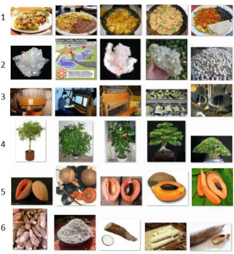
Figure 1: Which out-of-vocabulary nouns are plausible direct objects for the verb eat? Each row corresponds to a noun: 1. migas, 2. zeolite, 3. carillon, 4. ficus, 5. mamey and 6. manioc.
sponding classifier that scores noun arguments on the basis of various textual features. We use this discriminative framework to incorporate the visual information as new, visual features.
Our experiments evaluate the ability of these classifiers to correctly predict the selectional pref-erences of a small set of verbs. We evaluate two cases: 1) the case where the nouns are all as-sumed to be out-of-vocabulary, and the classifiers must make predictions without any corpus-based co-occurrence information, and 2) the case where we assume access to noun-verb co-occurrence in-formation derived from web-scale N-gram data.
We show that visual features are useful for some verbs, but not for others. For verbs taking abstract arguments without definitive visual features, the classifier can often learn to disregard the visual data. On the other hand, for verbs taking physi-cal arguments (such as food, animals, or people), the classifier can make accurate predictions using the nouns’ visual properties. In these cases, visual information remains useful even after incorporat-ing the web-scale statistics.
2 Visual Selectional Preference
Consider determining whether the nouns carillon, migas and mamey are plausible arguments for the
verb eat. Existing systems are unlikely to have such words in their training data, let alone infor-mation about their edibility. However, after in-specting a few images returned by a Google search for these words (Figure 1), a human might rea-sonably predict which words are edible. Humans make this determination by observing both intrin-sic visual properties (pits, skins, rounded shapes and fruity colors) and extrinsic visual context (cir-cular plates, bowls, and other food-related tools) (Oliva and Torralba, 2007).
We propose using similar information to pre-dict the plausibility of arbitrary verb-noun pairs. That is, we aim to learn the distinguishing vi-sual features of all nouns that are plausible argu-ments for a given verb. This differs from work that has aimed to recognize, annotate and retrieve objects defined by a single phrase, such as tree or wrist watch (Feng and Lapata, 2010a). These ap-proaches learn from labeled images during train-ing in order to assign words to unlabeled images during testing. In contrast, we analyze labeled im-ages (during training and testing) in order to deter-mine their visual compatibility with a given predi-cate. Our approach does not need labeled training images for a specific noun in order to assess that noun during testing; e.g. we can make a reason-able prediction for the plausibility of eat mamey even if we’ve never encountered mamey before.
We now specify how we automatically 1) down-load a set of images for each noun, 2) extract vi-sual features from each image, and 3) combine the visual features from multiple images into plausi-bility scores. Scripts, code and data are available at: www.clsp.jhu.edu/∼sbergsma/ImageSP/.
2.1 Mining noun images from the web
2.2 Extracting visual features from images
A range of features have been developed in the vi-sion community, typically with the aim of improv-ing content-based image retrieval (Deselaers et al., 2008). We follow previous work in using features in a bag-of-words representation that ignores the spacial relationship between image components.
Color Histogram Our first set of features are extracted from the color histogram of the image. We partition the color space by dividing the R, G, and B values of the pixel colors into equal-sized bins. For a given image, we count the number of pixels that occur within each RGB bin. Each color bin and its count is used as a feature dimension and its value, respectively. We describe how we choose the number of bins in Section 3.
SIFTKeypoints Additional features are derived from the image’s SIFT (scale-invariant feature transform) keypoints (Lowe, 2004). SIFT
key-points are detected at visually-distinct image loca-tions. Each keypoint has a corresponding descrip-tor vecdescrip-tor that identifies a location’s unique visual properties. SIFTkeypoints are conceptually simi-lar to local features identified by so-called corner detectors. Corner detectors find image locations that have “large gradients in all directions at a pre-determined scale” (Lowe, 2004). Unlike typical corner detectors, SIFT keypoints are invariant to scaling and rotation. They are also robust to illu-mination, noise and distortion. We identify SIFT
keypoints using David Lowe’s software: www.cs. ubc.ca/∼lowe/keypoints/. SIFT keypoints are taken from images converted to grayscale.
Since each keypoint is itself a vector, we quan-tize the keypoints by mapping them to a set of K discrete visual words. This set of words forms the visual vocabulary of our bag-of-words representa-tion. The set of words is obtained by clustering a random selection of keypoints into K cluster cen-troids using the K-means algorithm. The final ture representation for an image consists of a fea-ture dimension for each visual word; each feafea-ture value is the number of keypoints in the image that have that word as their nearest centroid.
We generate different clusterings (and thus dif-ferent vocabularies) separately for each verb pred-icate. For each verb, we randomly sample 500,000 keypoints from the set of downloaded images for that verb’s potential argument nouns, and run the clustering over these keypoints. Section 3
de-scribes how we choose the number of clusters, K.
2.3 Combining features with the DSPmodel We use DSP (Bergsma et al., 2008) to generate a plausibility score for a verb-noun pair, (v, n). Let
Φbe a function that generates features for nouns,
Φ : n → (φ1...φk). We explain below how, for
eachn, we aggregate visual features across multi-ple images to create features inΦ(n). DSP deter-mines whether nis a plausible argument ofv by scoring Φ(n)using a verb-specific set of learned weights, wv=(w1...wk). The weights are trained
for eachv in order to distinguish the verb’s posi-tive nouns from its negaposi-tives in training data (the generation of training data is also explained be-low). The weights can be learned using any bi-nary classification algorithm; we use logistic re-gression. At test time, we generate a final compat-ibility score (prediction) via the logistic function:
Score(v, n) = exp(wv·Φ(n)) 1 +exp(wv·Φ(n))
(1)
Our discriminative model differs from a recent generative model over words and visual features by Feng and Lapata (2010b). In that work, includ-ing visual features resulted in better topic clusters, which indirectly improved (topic-derived) word-word associations. In our work, visual features are directly exploited by a discriminative model, allowing us to use arbitrary and potentially inter-dependent visual attributes in our representation.
Generating Examples We follow Bergsma et al. (2008)’s approach by first calculating the point-wise mutual information (PMI) between predicate verbs and (direct object) argument nouns in a large parsed corpus. For each verb predicate, v, we cre-ate positive examples, (v, n), by pairing v with all nouns, n, such that v and n have a positive PMI, i.e. PMI(v, n) > 0. For each of these positives pairs (e.g. eat pasta), we generate two pseudo-negative examples, (v, n′), by randomly
pairing v with some nouns n′ that either did not
occur with v (and hence PMI is undefined) or have PMI(v, n′) ≤ 0 (e.g., eat distribution, eat
wheelchair). As in Bergsma et al. (2008), pseudo-negativesn′are chosen to have similar corpus
fre-quency to the original positive noun,n.
each v separately from all other verbs. For each
v, we take 85% of examples for training, 7.5% for development, and 7.5% for final testing.
Generating Features The DSPmodel allows us to use any information that might indicate a noun’s compatibility with a verb; we simply encode this information as features in the noun’s feature rep-resentation,Φ(n). Bergsma et al. used DSP’s flex-ibility to include novel string-based features of the noun argument (e.g., the verb become prefers lower-case direct objects; accuse prefers capital-ized ones). We augmentΦ(n)with visual features. Since we download multiple images for each noun, n, we have multiple color histograms and multiple bags ofSIFTkeypoints. To generate a sin-gle feature representation, Φ(n), we first sum the color and SIFT-keypoint feature vectors, respec-tively, across all the images inn’s image set. We then normalize each sum vector to unit length, and include all of the resulting normalized features as additional features inΦ(n).
In summary, we can produce a score for a(v, n)
pair at test time as follows: 1) select the appropri-ate weights,wv, for verb v, 2) generate the
com-posite (normalized) feature vector,Φ(n), for noun
n, and 3) score the features with the weights using the formula for Score(v, n)(Equation (1) above). In practice, this score is exactly what is returned by our logistic regression software package. We can use this score directly, or, for hard classifica-tions, predict positive if the returned probability is greater than 0.5 and otherwise predict negative.
3 Experimental Set-up
Task and Data The task is to predict whether a particular verb-noun pair, previously unseen dur-ing traindur-ing of the DSPclassifier, is a positive or a negative example, as defined in Section 2.3 above. We evaluate using Accuracy: the proportion of ex-amples correctly classified on test data. We calcu-late significance using McNemar’s test.
Since the negatives are pseudo-negatives, this kind of evaluation is also known as a pseudo-disambiguation evaluation. While the set-up of pseudo-disambiguation evaluations has varied in NLP (Chambers and Jurafsky, 2010), we use an identical set-up to Bergsma et al. (2008): we gen-erate positive and negative examples for DSPfrom a parsed and processed copy of the AQUAINT cor-pus, and use the same PMI-threshold (i.e. 0) and positive-to-negative ratio (i.e.1:2).
We evaluate on nouns in the direct object po-sition of seven verbs: eat, inform, hit, kill, park, hunt and shoot down. The total number of training examples for these verbs varies from roughly 500 to 10,000 instances, while the number of test in-stances varies from roughly 50 to 1000 inin-stances.
We chose these seven verbs as test cases be-cause we speculated they might benefit from vi-sual information to different degrees (e.g. we ex-pected indicative food-features for eat, but perhaps less helpful human-features for inform, etc.). Ide-ally one would like to automaticIde-ally categorize all the verbs for which visual features might be help-ful, but it is natural to first demonstrate the bene-fits of visual information in certain cases in order to motivate further study. Importantly, note that while we hand-selected a set of verb predicates, our evaluation data is based on real observed ar-guments of these predicates, and in particular not on nouns for which we would a priori expect vi-sual information to be predictive. Our evaluation is thus focused, but realistic.
Classifier In all cases, we use an L2-regularized logistic regression model for DSP’s base classifier, and train it via LIBLINEAR(Fan et al., 2008). We optimize the regularization parameter on the de-velopment data.
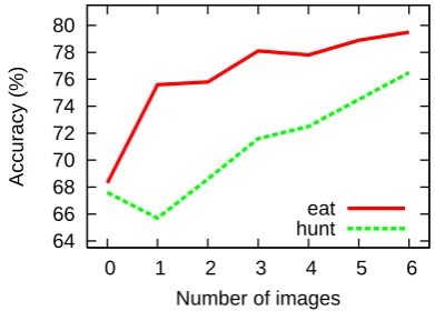
Visual Features For each noun,1 we take the first six images returned from both Google and Flickr, and extract the corresponding visual fea-tures as described above. While we later discov-ered that the more images we have, the better the results (Figure 2), we initially decided to use only six images mainly for computational reasons; downloading and processing images is space and time-intensive.
Rather than selecting fixed values for the size of the color bins and the number of SIFT centroids, we take advantage of our model’s flexibility to use features over different granularities: we use sepa-rate features with both 64 and 512 color bins, and with both 100 and 1000SIFTcentroids. The
flexi-bility to include visual information at different lev-els of granularity is one of the chief advantages of the discriminative model.
Test Configurations We are primarily inter-ested in whether visual information can lead to
1For a given verb in our corpus, D
System eat inform hit kill park hunt shoot down Average
Baseline 68.3 68.0 68.7 67.7 69.9 67.6 70.0 68.6
+ Visual Features via Flickr 75.8 68.0 68.8 67.2 69.9 69.6 70.0 69.9 + Visual Features via Google 79.5 68.2 68.7 68.5 69.9 76.5 72.0 71.9
Table 1: Using visual features from Google significantly improves accuracy (%) over the baseline system on eat (p<0.001), kill (p<0.1) and hunt (p<0.1).
better predictions on out-of-vocabulary (OOV) nouns, but obtaining a sufficiently-large test set of labeled OOV instances is difficult. We therefore first provide results on simulated OOV arguments (Section 4.1), where we assume no corpus-based knowledge is available to the DSP classifier. That is, we initially exclude corpus-based features from our models. We compare visual models to ones that only use features for the noun string (such features are always available). Our string features are binary features that indicate the ‘shape’ of the noun via the regular expression maps: [A-Z]+→
A, and [a-z]+→a. E.g., Al Unser Jr. will have the one feature ‘Aa Aa Aa.’.
In the second part of our results (Section 4.2), we test whether visual information can help even in the presence of high-quality corpus-based fea-tures. We use Keller and Lapata (2003)’s approach to obtain web-scale co-occurrence frequencies for the verb-noun pair. That is, we retrieve counts for the pattern “V Det N” from a web-scale Google N-gram corpus (Lin et al., 2010). Here, Vis any inflection of the verb, Det is the, a, an, or the empty string, and Nis the noun. We include the log-count of this pattern as a feature, and also in-clude separate features for the log-counts of the noun and verb themselves. By multiplying these features by appropriate weights, a classifier can generate a (web-based) PMI score.
4 Results
4.1 Results on OOV nouns
We now compare the use of visual features to string-based features alone (Baseline), simulat-ing out-of-vocabulary arguments by assumsimulat-ing no corpus-based knowledge is available for the noun features. For these verbs, we actually found the Baseline with only string features to be no better than picking the majority-class.
Visual features significantly improve perfor-mance for 3 of the verbs (Table 1). Visual fea-tures do not improve (but also do not impair) ac-curacy on the verbs that have mostly abstract or
64 66 68 70 72 74 76 78 80
0 1 2 3 4 5 6
Accuracy (%)
Number of images eat hunt
Figure 2: The more images, the more accurate: Performance on the verbs eat and hunt as features are extracted from a varying number of images.
general arguments. For example, one can “hit tur-bulence,” “hit record,” or “hit the slopes,” but there are no visual features that can help select these nouns. Macro-averaged accuracy across all verbs increases from a baseline of 68.6% to 71.9% using Google-derived visual features.
The features obtained from Google images per-form better than features from Flickr (Table 1). In-specting the retrieved image sets, we observe that compared to Flickr, Google tends to retrieve more consistent, more canonical images for a particular noun. For example, Google’s top results for the query “buffalo” are exclusively images of buffalo animals. On Flickr, “buffalo” returns images of the city of Buffalo, buffalo hides, and pictures of buffalo animals alongside people, cars, birds, etc. For our purposes, the consistency of the Google images is better; it makes learning and predicting easier for the visual classifier.
We provide further analysis using Google ages only. Figure 2 shows that, as we use more im-ages, accuracy on the verbs eat and hunt improves and is not yet leveling off. With computation only linear in the number of images, adding even more images is one possible way to improve accuracy.
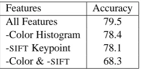
Features Accuracy All Features 79.5 -Color Histogram 78.4 -SIFT Keypoint 78.1
-Color & -SIFT 68.3
Table 2: Accuracy on eat as different feature classes are removed.
0.3 0.4 0.5 0.6 0.7 0.8 0.9
0 1 2 3 4 5 6 7
Visual Selectional Preference
Human compatibility judgement group
husband debt
local people
villagercost
egg
apple pizza
lunch meal
Figure 3: Visual selectional preference correlates well with human judgments: arguments of the verb eat are plotted using visual and average hu-man compatibility scores.
the verb eat. Either visual feature type helps a lot on its own; together they further improve accuracy. We also tried replacing our logistic classifier with kernelized SVMs, which have previously proved useful for object recognition (Chapelle et al., 1999). While kernel-SVMs can implicitly con-sider all combinations of features (resulting in the encoding of richer visual information), we found the resulting gains over linear classifiers to be min-imal. The kernelized SVMs also took much longer to train and apply. The further development of ef-fective while still efficient visual features remains an important direction for future work.
Figure 3 compares the scores of the visual system (computed via Equation (1)) to human plausibility judgments (described by Pad´o et al. (2006)).2 The human scores are the average judg-ments for the question, “how common is it to eat X?” where X is a given noun. Participants re-sponded with scores from 1 (very uncommon) to 7 (very common). These average judgments have a high correlation with our predicted scores; the
2Available online at http://www.nlpado.de/
∼ulrike/data/pado plausibility.tgz
System eat kill hunt
Baseline 68.3 67.7 67.6
+ Visual Features alone 79.5 68.5 76.5 + Web Co-occ alone 85.1 74.0 76.5 + Web Co-occ & Visual 85.7 74.3 78.4
Table 3: Visual features improve accuracy (%) even when web co-occurrence information is used.
Pearson correlation coefficient is 0.803. The vi-sual system does a good job on the nouns egg, meal, pizza and apple, but ranks debt above (the somewhat abstract) lunch. Looking at the Google images for lunch, we note that clearer pictures of food occur beyond the top 6 images, and hence us-ing more images would likely improve scorus-ing.
Finally, we note that for eat, we found the visual system’s accuracy was consistent across nouns of different frequencies. This contrasts with systems using text-based features; these perform much bet-ter on more frequent nouns (Bergsma et al., 2008).
4.2 Results with web-scale statistics
We have shown that visual information can result in significantly improved performance in cases where no corpus-based information is available. Do these gains hold up when high-quality corpus-based information is available?
On those verbs where visual information helped in the OOV setting, visual information remains helpful even with features encoding web-scale co-occurrence statistics (Table 3).3 Note the gains from adding visual features are consistent in all three cases, but not statistically significant, as the proportion of nouns where the visual features can help is now much smaller.
These final results are somewhat sobering. Vi-sual information is not helpful for every verb, and even in the positive cases, it is not very helpful when combined with existing text-based features. However, the exploitation of visual information is still in its infancy in NLP. Using search engines to obtain images for NLP today is perhaps similar to how search engines were also used to obtain web-scale text statistics for NLP a decade ago. While we leveraged a relatively small number of visual features from a relatively small number of images,
future advances in computer vision and large-scale data processing will allow richer visual informa-tion to be extracted and applied to NLP problems.
5 Conclusion
We have shown that it is possible to predict verb-noun selectional preference purely on the basis of visual information. For a given noun, web images are downloaded, processed, and then analyzed by classifiers corresponding to different verbs. Each verb classifier is trained to identify the visual properties that distinguish the verb’s preferred ar-guments. Statistically-significant improvements were obtained on three verbs and visual data re-mains helpful even in the presence of high-quality web-scale co-occurrence information.
These results give us a good basis for mov-ing forward. We know where we should get our images (Google), which features are useful (both color and SIFT) and how many images to use (as many as possible). It remains to be seen which other predicates, which other predicate-argument relationships, and which other NLP problems can benefit from visual information.
References
S. Bergsma and B. Van Durme. 2011. Learning bilin-gual lexicons using the visual similarity of labeled web images. In Proc. IJCAI.
S. Bergsma, D. Lin, and R. Goebel. 2008. Discrimi-native learning of selectional preference from unla-beled text. In Proc. EMNLP, pages 59–68.
N. Chambers and D. Jurafsky. 2010. Improving the use of pseudo-words for evaluating selectional pref-erences. In Proc. ACL, pages 445–453.
O. Chapelle, P. Haffner, and V. Vapnik. 1999. Support vector machines for histogram-based image classi-fication. IEEE Transactions on Neural Networks, 10(5):1055–1064.
S. Clark and D. Weir. 2002. Class-based probabil-ity estimation using a semantic hierarchy. Computa-tional Linguistics, 28(2):187–206.
I. Dagan and A. Itai. 1990. Automatic processing of large corpora for the resolution of anaphora refer-ences. In Proc. COLING, pages 330–332.
I. Dagan, L. Lee, and F. C. N. Pereira. 1999. Similarity-based models of word cooccurrence probabilities. Mach. Learn., 34(1-3):43–69.
T. Deselaers, D. Keysers, and H. Ney. 2008. Features for image retrieval: an experimental comparison. In-formation Retrieval, 11:77–107.
K. Erk. 2007. A simple, similarity-based model for selectional preference. In Proc. ACL, pages 216– 223.
R.-E. Fan, K.-W. Chang, C.-J. Hsieh, X.-R. Wang, and C.-J. Lin. 2008. LIBLINEAR: A library for large linear classification. Journal of Machine Learning Research, 9:1871–1874.
Y. Feng and M. Lapata. 2010a. Topic models for im-age annotation and text illustration. In Proc. HLT-NAACL, pages 831–839.
Y. Feng and M. Lapata. 2010b. Visual information in semantic representation. In Proc. HLT-NAACL, pages 91–99.
R. Fergus, L. Fei-Fei, P. Perona, and A. Zisserman. 2005. Learning object categories from Google’s Im-age Search. In Proc. ICCV, pIm-ages 1816–1823.
D. Hindle and M. Rooth. 1993. Structural ambigu-ity and lexical relations. Computational Linguistics, 19(1):103–120.
F. Keller and M. Lapata. 2003. Using the web to ob-tain frequencies for unseen bigrams. Computational Linguistics, 29(3):459–484.
D. Lin, K. Church, H. Ji, S. Sekine, D. Yarowsky, S. Bergsma, K. Patil, E. Pitler, R. Lathbury, V. Rao, K. Dalwani, and S. Narsale. 2010. New tools for web-scale N-grams. In Proc. LREC, pages 2221– 2227.
D. G. Lowe. 2004. Distinctive image features from scale-invariant keypoints. IJCV, 60:91–110.
D. ´O S´eaghdha. 2010. Latent variable models of se-lectional preference. In Proc. ACL, pages 435–444.
A. Oliva and A. Torralba. 2007. The role of context in object recognition. Trends in Cognitive Sciences, 11(12):520–527.
U. Pad ´o, F. Keller, and M. Crocker. 2006. Combining syntax and thematic fit in a probabilistic model of sentence processing. In Proc. CogSci, pages 657– 662.
P. Resnik. 1996. Selectional constraints: An information-theoretic model and its computational realization. Cognition, 61:127–159.
P. Resnik. 1997. Selectional preference and sense dis-ambiguation. In Proc. ACL SIGLEX Workshop on Tagging Text with Lexical Semantics: Why, What, and How?
A. Ritter, Mausam, and O. Etzioni. 2010. A latent dirichlet allocation method for selectional prefer-ences. In Proc. ACL, pages 424–434.