University of South Carolina
Scholar Commons
Theses and Dissertations
8-9-2014
Network Analysis and Cluster Detection Using
Markov Theory
John William Campbell
University of South Carolina - Columbia
Follow this and additional works at:https://scholarcommons.sc.edu/etd
Part of thePhysics Commons
This Open Access Thesis is brought to you by Scholar Commons. It has been accepted for inclusion in Theses and Dissertations by an authorized administrator of Scholar Commons. For more information, please [email protected].
Recommended Citation
Campbell, J. W.(2014).Network Analysis and Cluster Detection Using Markov Theory.(Master's thesis). Retrieved from
Network Analysis and Cluster Detection Using Markov Theory
by
John William Campbell
Bachelor of Science Wofford College 1994
Bachelor of Arts Wofford College 1994
Submitted in Partial Fulfillment of the Requirements
for the Degree of Master of Science in
Physics
College of Arts and Sciences
University of South Carolina
2014
Accepted by:
Joseph E. Johnson, Director of Thesis
Matthias Schindler, Reader
c
Copyright by John William Campbell, 2014
Abstract
Networks are a vital part of nature and society, yet many aspects of how networks
function are still largely unknown. From understanding the internet to biology,
chem-istry, and physics, networks play a role, but even some of the most basic questions
about networks can be difficult to answer. How are two networks alike or different?
How do networks within networks form and how can clusters be detected? As
net-works change with time, how can we monitor those changes? The answers to these
questions are vitally important to humans’ understanding of the world. Better
under-standing of networks allows for things like more efficient electrical distribution grids
and more reliable real-time network intrusion detection systems. It also allows for a
better understanding of how nature forms networks like the bonds that form molecules
and the networks that carry water from the mountains to the sea and back again.
Network analysis and cluster detection is a dynamic area of mathematics featuring
many different approaches. This research is intended to approach network analysis
using Markov matrices and methods normally reserved for physical systems. Three
methods were used in this project to illuminate network classification and behaviors:
multi-order Renyi entropy comparisons, eigenvalues/eigenvectors analysis to detect
network clusters, and property tables used to create networks with clusters. All three
methods produced promising results and hint that this new way of viewing networks
Table of Contents
Abstract . . . iii
List of Tables . . . v
List of Figures . . . vi
Chapter 1 Introduction . . . 1
Chapter 2 The Connection Matrix and Markov Monoids. . . 7
Chapter 3 Renyi Entropy of Networks . . . 12
Chapter 4 Eigenvalue Clustering . . . 21
Chapter 5 Property Clustering . . . 26
Chapter 6 Conclusion . . . 31
List of Tables
Table 3.1 Comparison of Sample Network To Known Topologies . . . 14
List of Figures
Figure 3.1 10-Node Ring Network: Every node connected to two neighbors . 16
Figure 3.2 10-Node Cluster Network: Every node connected to every other node 17
Figure 3.3 10-Node Tree Network: Three-level tree . . . 18
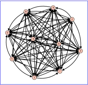
Figure 3.4 9-Node Network with 4 Symmetric Clusters . . . 19
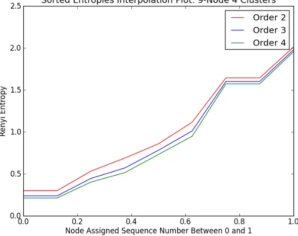
Figure 3.5 Entropy Spectra of 9-Node Network shown in Figure 3.4 These are the interpolation functions between 0 and 1 for Renyi en-tropies of order 2, 3, and 4 (I2,I3, I4) . . . 20
Figure 4.1 10-Node Cluster Network: 3 clusters . . . 25
Figure 5.1 Discovered Elements Cluster 1 . . . 29
Figure 5.2 Discovered Elements Cluster 2 . . . 29
Chapter 1
Introduction
Networks are everywhere and effect the lives of everyone on Earth on a daily basis.
Telecommunication networks route data to people next door or to people on the
other side of the planet in fractions of a second. Financial networks that transfer
money from one person or organization to another are the backbone of the world
economy. The modern technological age would not be possible without electrical
networks that power the infrastructure upon which the world depends. The entire
planet is more accessible than it has ever been in history because of the complex
transportation networks that take people from one point to another. Those are just
a few of the obvious world-wide structures that people think of when they think of
networks. There are however, more subtle networks that are not as obvious to most
people. As pointed out by Singer, the branching structure of leaves and the network
of blood vessels in the human body are but two examples of nature forming nested
loop networks to resist damage [8]. McVittie suggests that even genes and cells are
better understood in terms of networks [9]. A deeper understanding of networks can
assist the scientist in better understanding nature, but can also help prevent failures
like internet outages and power failures, according to Bashan et. al. [10], and make
the city bus system more efficient and more economical. Even though all of these
networks are very different, Sinha shows that there are certain universal principles
that govern core network structure and behavior [11]. This research is an attempt to
discover some of these core principles.
strengths of the connections between these nodes. The nodes themselves can be
ar-bitrarily numbered from 1 to N. The term "strength of connection" can have many
meanings depending on what type of network is being described. For example, the
strength of connection between people on a social network could be defined as the
number of messages exchanged during a certain time period. The strength of
con-nection between two airports could be defined as the number of passengers traveling
from one to the other in a given day or perhaps the total number of flights from one
to the other. It is important to note that, depending on the definition, the network
may or may not be symmetric. In the example of the airports, there may be far
more flights from airport A to airport B than from airport B to airport A. So the
A to B connection would be much stronger than the B to A connection. Once the
definition of the strength of connection is determined for a given network, it is simple
to represent the network with a matrix, referred to in this paper as the connection
matrix,Ci,j. The element in the ith row andjth column is the strength of connection
from nodej to nodei. Note that the strength of connection is always a positive value.
To denote a connection incoming to node j from node i, the strength of connection
value should go in the jth row and ith column. In each case, the column represents
the source node and the row the destination node. If the strength of connection does
not have a directionality, then thei, j element will be the same as thej, ielement and
the matrix will be symmetric. Following this prescription for building the connection
matrix, leaves the diagonal elements of the matrix undefined since it makes no sense
to describe the strength of connection of a node to itself. Since the diagonal is
un-defined, the Ci,j matrix is an ambiguous mathematical entity. It has no eigenvalues,
eigenvectors, nor an inverse. The solution to this problem with the Ci,j matrix is
to model the network using Markov monoids. This process is described in the next
chapter.
connec-tivity of things is one of the most difficult mathematical domains. First, there is no
useful classification system for large and complex networks. According to Meador,
for simple networks, labels such as ring, tree, star, bus, and mesh can be applied [12]
and are mainly used in the realm of computer networking, but even slight
complex-ity can lead to ambigucomplex-ity in labeling. Structures like trees of stars or rings of trees
can occur. When it comes to large networks like power grids or air traffic however,
there is no satisfactory way to classify them. Computer network topologies to which
a label can be applied were designed to be that type of topology for functional
rea-sons. Classifying a large, complex network that arises through natural or man-made
processes as being composed of the labeled topology types may help aid in
under-standing why that network formed in the way that it did. Second, there is not even a
method to uniquely define a network. Since the nodes can be arbitrarily numbered,
for a given network with N nodes, there are N! ways to describe that network with
a Ci,j matrix. Thus not only is it difficult to compare two networks, it is hard to
take two Ci,j matrices and tell if they describe the same network or not. One
impor-tant problem that depends on the solution of the problem of comparing networks is
comparing a network to itself at two different times. This is important to allow the
study of the evolution of a network over time to detect intrusions or other network
problems. Finally, detecting clusters, tightly interconnected subnetworks within
net-works, is a problem that has no accepted method of solution. Estivill-Castro describes
many algorithms for finding clusters [6] such as connectivity-based, centroid-based,
distribution-based, and density-based algorithms. Many of these methods, however,
are heavily dependent upon a certain type of network definition and there are no
accepted ways to evaluate the effectiveness of the analyses. The work described in
this paper approaches solving all of these problems by first fixing the ambiguity in
the Ci,j matrix. Then, more traditional analysis methods can be brought to bear on
There are other computer network analysis methods that attempt to detect
anoma-lies in network traffic and to model networks as Markov processes. Intrusion detection
systems (IDS) continue to rise in importance on today’s networks as more and more
of the world’s business moves online. As targets become more valuable, attempts
to penetrate modern protection systems skyrocket. Callagari states that the goals
of modern hackers include eavesdropping, downloading unauthorized information,
tampering, spoofing, flooding networks to cause service disruptions, injecting
mali-cious code, exploiting code flaws, and cracking passwords just to name a few [18].
To mitigate these attacks, there are two types of IDS as described by Brindasri et.
al.: signature-based IDS (SBIDS and anomaly-based IDS (ABIDS) [16]. The SBIDS
method works only against known attacks. Improving the ABIDS systems offers hope
of detecting yet unused attacks as they happen. Network comparisons over time are
the basis for ABIDS. Budalakoti’s work shows how these methods learn the networks
normal profile and alert on the deviations from that profile (anomalies) [17] while
at-tempting to minimize false positives. Bedajena and Rout attempt to detect network
intrusions by modeling networks using hidden Markov models and detecting changes
in probablilities of transitions between nodes [15]. The occurrence of low probability
events is indicative of an anomaly and a possible intrusion [16]. The analysis work
described in later chapters here use volume or counts of messages from one node to
another, but Diaz et. al. suggest that this Markov modeling technique can be used at
the protocol level by looking at the messages themselves or the sequence of messages
[19].
Fortunato points out that detecting clusters, or community structures in networks
is important to any area of study where systems are represented by graphs [21].
Un-derstanding the nodes and structure of clusters goes a long way toward unUn-derstanding
the efficiencies (or inefficiencies) or a structure along with its vulnerabilities. For
particular importance. Despite the importance of the problem, there are problems
with the solution that result in a great number of methods attempting to solve it.
Fortunato’s work also suggests that the biggest obstacle to a solution is the fact that
the elements of the problem are not rigorously defined, resulting in arbitrariness of
the methods and solutions [21]. No definition of a cluster is universally accepted [21]
and often depends on the system being analyzed. According to Fortunato, after a
paper by Girvan and Newman in 2002 [22] [21], brought great interest to the field
of cluster detection in 2002, many physicists became interested and brought to bear
their analytical techniques. In their paper, Girvan and Newman discuss the
tradi-tional method of cluster detection, hierarchical clustering, and their new proposed
method, edge betweenness and community structure [22]. In hierarchical clustering,
vertices are weighted and then edges are added one by one in order of strongest to
weakest pairs causing clusters to appear. The ambiguity in this method lies on how
to define the weights for the nodes to begin with. In the edge betweenness method,
Girvan and Newman reverse the process by instead removing weak edges from a
graph to eventually reveal the communities underneath. Hassan et. al. describe two
categories of cluster detection methods: supervised and unsupervised [20]. In
super-vised clustering, an algorithm learns using a training dataset and then applies this
algorithm on the actual data. In unsupervised cluster detection, no training set is
used. Sometimes, both types of algorithms are used together. In some methods, the
number of clusters must be decided beforehand and in others, the number of clusters
is determined by the algorithm. Moradi et. al. point out how the sheer number of
methods used for cluster detection combined with the lack of universal definitions of
clusters and their components makes grading detection algorithms very difficult [23].
In this work, an attempt has been made to remove some of the ambiguity of
defining the rules for creating the connection matrix by using raw weights or counts
monoid from the connection matrix. Then in Chapter 3, that Markov monoid is used
to calculate the entropy spectrum of the network in order to identify changes in the
network and to classify networks. In Chapter 4, the eigenvalues and eigenvectors of
the Markov monoid are used to discover clusters in the network. Finally, in Chapter
5, a special method is outlined for constructing the connection matrix from a list of
Chapter 2
The Connection Matrix and Markov Monoids
A network is defined as a set of nodes with connections between the nodes. The
anal-ysis methods used in this project rely on first forming a connection matrix, referred
to as Ci,j, that describes the relative strength of connections between the nodes i
and j. The method by which Ci,j is formed is dependent upon the application, but
the end result is that Ci,j describes the strength of the connection between nodes i
and j where i, j = 1,2, ...N. The element Ci,j is a non-negative number, and the
diagonal of Ci,j is undefined since it refers to a node’s connection to itself. It is also
important to point out that since the element Ci,j can be any positive real number,
it contains more information about the connection than a graph (where the elements
of Ci,j are limited to the values 1 and 0), and so the connection matrix may not be
symmetric. Analyzing and comparing different networks using connection matrices
is difficult because of the fact that there is no natural way to order the nodes. For a
network ofN nodes, there are N! ways to order the nodes and thusN! Ci,j matrices
that describe the same network. The goal of this research is to develop methods of
analysis that identify the defining characteristics of a network, regardless of the
spe-cific representation, in the same way that series expansions can describe the dominant
components of complex phenomena.
To begin, the Ci,j matrix for a complex system of nodes is considered analogous
to a state vector for a simpler system, except for one problem. The diagonal ofCi,j is
undefined. To allow further analysis of the network using the Ci,j matrix, it is useful
specifically, the Markov monoid.
The general linear group, GL, contains many of the groups in physics and is
composed of the set of all n ×n invertible matrices and the operation of matrix
multiplication. It was shown by Johnson [1] that the general linear group in N
dimensions can be decomposed into the Markov type Lie group and an abelian scaling
group. That is to say that GL=A+M where A=eaiAi and M =eλi,jLi,j Here, the
Ai are the basis matrices in the abelian scaling group algebra and the Li,j (i 6= j)
are the basis matrices in the Markov-type Lie group Lie algebra. In N dimensions,
there are N abelian group algebra elements and N2 −N Markov-type Lie algebra
components. The abelian group algebra basis matrices are matrices that have a 1 in
the i, i position and zeros elsewhere. For example, for the 3×3 basis, the abelian
group basis matrices are:
A1 =
1 0 0
0 0 0
0 0 0
A2 =
0 0 0
0 1 0
0 0 0
A3 =
0 0 0
0 0 0
0 0 1
When a member of the abelian group operates on a vector, it simply shrinks or
stretches a vector along one or more axes. By varying the coefficients that multiply
each basis matrix, any combination of stretching or shrinking along any of thenaxes
can be accomplished: G(a) = eaiAi.
The Li,j Lie algebra basis matrices have a 1 in the i, j position and a −1 in the
j, j position. In other words, whichever column contains the 1 also has a −1 on the
diagonal in that same column. The 3×3 basis matrices for the Markov-type Lie
algebra are
L1,2 =
0 1 0
0 −1 0
0 0 0
L1,3 =
0 0 1
0 0 0
0 0 −1
L2,1 =
−1 0 0
1 0 0
0 0 0
L2,3 =
0 0 0
0 0 1
0 0 −1
L3,1 =
−1 0 0
0 0 0
1 0 0
L3,2 =
0 0 0
0 −1 0
0 1 0
The Markov-type Lie group preserves the sums of the components of any vector
it acts upon (in contrast to a rotation which preserves the sum of the squares).
It preserves a linear form rather than a quadratic form. However, it can take a
vector with only non-negative components into a vector with negative components.
In Strang’s book, he describes how a real Markov transformation must preserve the
non-negative nature of the elements of the vector that it acts upon [13]. Johnson
showed that this requirement can be met by restricting the λi,j coefficients to be
non-negative. The Markov monoid is defined as
M(λ) = eλi,jLi,j (2.1)
where theλi,j are non-negative. The Markov monoid represents a true Markov
trans-formation. The fact that it is monoid means that the transformation has no inverse as
is required by Markov processes. Markov transformations have no inverse since they
represent irreversible diffusion and work by transferring a non-negative fraction of
some quantity from one node to another during each transformation operation while
preserving the sum of the vector’s components. As an example, look at the following
Markov monoid using only the first two terms of the exponential expansion:
L= 0.5L1,2+ 0.2L2,1 =
−0.2 0.5
0.2 −0.5
M(λ= 1) =I+ 1L=
0.8 0.5
0.2 0.5
X1 =M X0 =
0.8 0.5
0.2 0.5
10 10 = 13 7
X2 =M X1 =
0.8 0.5
0.2 0.5
13 7 =
13.9
6.1
It is clear that for each operation, 50% of node 2 is transferred to node 1 and 20%
of node 1 is transferred to node 2. Applied to a physical process, this transformation
represents an irreversible diffusion with the transfer rates from one node to the other
described by the Markov monoid. Note that the sums of the columns of the Markov
monoid are always 1. Note also that this transformation represents only a
redistri-bution of the quantities described in the state vector since the sum of the elements
of the state vector remains unchanged after the transformation. Nothing is added or
taken away. This can be visualized as an aquarium of water divided by a membrane
with two, one-direction outlets placed in the membrane. According to the Markov
monoid description, if dye is placed on one side of the membrane, the distribution of
the dye will eventually reach an equilibrium state. Each successive application of M
decreases the amount of information and increases the entropy of the system as the
system moves toward equilibrium.
It was proven by Johnson [3] that every network corresponds to exactly one
Markov monoid Lie generator and vice versa. Thus they are isomorphic. Each
net-work corresponds to a family of Markov transformations. That paper showed that
the Lie algebra monoid generated all Markov transformations that are continuously
connected to the identity. To useCi,j to form a Markov monoid, set λi,j =Ci,j for the
off diagonal terms and let the Li,j define the diagonals. The result is a Lie algebra
element,
with the elements of Ci,j on the off-diagonals and the negative of the column sums
on the diagonal. The Markov monoid transformation is then
M =eλL (2.3)
where λ is just a positive constant. So the network described by Ci,j defines a Lie
algebra elementLwhich generates a Markov monoid transformation with the
param-eter λ. This M has a well defined diagonal and models the original network as a
series of flows from one node to another at rates given by the connection matrix and
described by this Markov process. In the expansion of M
M =I+λL+ 1 2!(λL)
2+ 1
3!(λL)
3+... (2.4)
the L term represents direct connections between nodes, the L2 term the secondary
(node through a node) connections, and so on. The one precaution that must be
taken is to choose λ so that the the expansion will not overpower the unit matrix.
The resulting M matrix has a well defined diagonal and thus can be used for
en-tropy calculations and eigenvalue / eigenvector analysis as Johnson demonstrated.
The columns of M are non-negative and sum to one and thus can be thought of as
probability distributions. By modeling a network as a series of flows from one node
to another, the problem of the ambiguity of the Ci,j matrix undefined diagonal has
been overcome and new avenues of analysis have been opened. These methods of
Chapter 3
Renyi Entropy of Networks
The ability to compare two networks is essential for two different types of inquiries.
The first type is the comparison of two completely different networks to discover
sim-ilarities. This type of analysis can be used to compare two corporations to determine
if one is more similar to successful structures or to less successful ones. It can be used
to compare the industrial outputs or other economic properties of countries. Johnson
suggests that power grids and data infrastructure can be analyzed as viewed from the
perspective of networks to determine which plans are most efficient and most effective
[2]. In the second type of inquiry, a network can be compared to itself at different
times to determine if changes have taken place. This is useful for the detection of
problems such as hardware failures, sabotage, or network intrusion. Both types of
analysis approach the problem by comparing two networks.
Johnson’s work shows that the rows and columns of the M matrix described in
the previous chapter can be used to calculate an entropy spectrum for the network
described within [3][5]. According to Renyi, the jth order Renyi entropy, R
j of a row
or column of an N byN M matrix with ai as the elements of the row or column, is
calculated by [14]
Rj =
1
1−jlog2(
N
X
i=1
aij) (3.1)
The entropies for the row or column are then arranged in ascending order and used to
generate an interpolation function,Ij between 0 and 1. In other words, each entropy
value in the list of sorted entropies for a given order is associated with a point on a
interpolation function is generated to fit the N points (x, y) where x is the value of
the point on the number line andyis the entropy value. Ij, the interpolation function
for the jth order Renyi entropy, allows a comparison between the entropy spectra of
networks with different numbers of nodes. The sorting of the entropies assigns a
sequence to the nodes and eliminates arbitrary numbering of the nodes. The sort
order by node is saved and the subsequent entropy calculations use the same sort
order. For two different networks aand b, a measure of similarity of their network jth
order entropies, Qabj, can be obtained by choosing k equally spaced points between
0 and 1 and summing the square of the differences of the interpolation functions at
those points.
Qabj = k
X
i=1
((Ija(xi)−Ijb(xi))2) (3.2)
Using several orders of Renyi entropies for each network, an overall similarity measure,
Sab, can be obtained.
Sab =
4
Y
i=2
e−Qabi (3.3)
In this equation, the value ofi goes from 2 to however many orders of Renyi entropy
are included in the calculation. In this work, Renyi entropies of orders 2, 3, and 4
were used. Sab, referred to as the similarity quotient, is obviously 1 for networks with
identical entropy spectra and is lower the more the spectra differ. Using this method,
it is possible to compare unknown networks to simple representative networks of
known types. Expanding unknown networks in terms of known networks is analogous
to other analysis methods used in physics. Approximations using series expansions
such as Fourier analysis, Taylor series, and expansion in Hermite polynomials is a
fundamental concept in physics with the objective that lower order terms are more
important. Here, networks are expanded in powers of Renyi entropy and in terms of
known networks.
In this study, simple 10-node ring (Figure 3.1), cluster (Figure 3.2), and tree
Table 3.1 Comparison of Sample Network To Known Topologies
Representative Network Simlarity Quotient (Sab)
Ring 2×10⁻⁵
Cluster 6×10⁻⁶
Tree 0.162
It is illustrative to compare a slightly more complex network to these simple
known networks. In this case, a 9-node network with 4 symmetric clusters is used
(Figure 3.4) . The entropy spectra for the orders 2, 3, and 4 Renyi entropies for this
network are shown in Figure 3.5. Now using Equation 3.3, this unknown network can
be cast according to how similar it is to the known networks.
In this example case, in terms of entropy spectra, the unknown network is much
more similar to a representative tree network than to a ring or cluster (see Table 3.1).
This type of analysis is useful to get a feel for how a network is structured compared
to something that is easy to visualize.
Johnson has conjectured that, in principle, the connection matrix could be
gen-erated from multiple orders of the Renyi entropy, since the entropy spectra contain
the same information. In practice, however, this calculation would be very difficult
and was not attempted in this work.
This same method of calculating and comparing the entropy spectra of networks
allows for the comparison of a single network at different points in time. A change
in the entropy spectra of an optimal network could indicate a problem or at least a
change that needs attention. Under Johnson’s direction, this type of analysis on LAN
traffic was done as part of ExaSphere, a DARPA funded project by the Advanced
Solutions Group at the University of South Caroline in 2006, and has shown the
ability to detect anomalies with nontrivial numbers of nodes [4] [24].
Calculating multiple order Renyi entropies from the M matrix, sorting and
main-taining a sort order, and creating an interpolation function from these sorted
Figure 3.5 Entropy Spectra of 9-Node Network shown in Figure 3.4 These are the interpolation functions between 0 and 1 for Renyi entropies of order 2, 3, and 4 (I2,
Chapter 4
Eigenvalue Clustering
Estivill-Castro describes how there is no uniquely accepted method for detecting
clusters within networks [6]. Statistical analyses, distance definitions, and density
characterizations are but a few methods used to find clusters of nodes. In each
method, the definitions depend on the data sets and on the purpose of the analysis.
Furthermore, Farber et. al. point out that there is no accepted method for evaluating
the results of the analysis [7]. The approach used in this research is fundamental and
method agnostic, and thus can be used to derive clusters in any network in a single,
very natural intuitive way.
Since the Markov matrix M can be thought of as modeling an imaginary flow
among the nodes, Johnson conjectures that the eigenvalues and eigenvectors of this
matrix can be useful in discovering clustering structures within networks [5]. The
basis of this conjecture is that the flows modeled by the Markov matrix, generated by
the modified connection matrix, has eigenvalues that represent linear combinations
of nodes which collectively approach equilibrium at the rate of the corresponding
eigenvalue and achieve this with flows among those participating nodes [5]. That
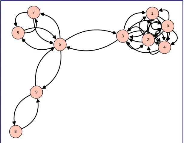
hypothesis is tested with two sample networks. They are both 10-node networks
with 3 main clusters (see Figure 4.1). In the first, the intracluster connections are
all the same strength with the connections between the clusters much weaker. The
second network is the same except for the fact that the 5-node cluster has a 3-node
cluster within it (nodes 0, 1, and 2 are more strongly connected than the others).
By creating a threshold value based on a set fraction of the maximum component
value of all of the eigenvectors and setting components below that threshold to zero,
the nodes corresponding to the remaining non-zero elements of the eigenvector are
members of a cluster. This is known by inspection after looking at the associated
eigenvalue. After applying the threshold function, the eigenvector associated with the
lowest eigenvalue contains 5 non-zero elements. These non-zero elements correspond
to the 5 nodes that are members of the strongest cluster in the network. Similarly,
in sequence, the other eigenvalues and their associated non-zero eigenvector elements
point out the other clusters. As the eigenvalues get larger, the cluster, pointed out
by the non-zero eigenvector elements, gets weaker. Finally, the 3 largest eigenvalues
are very near 1. The nodes included by looking at their associated eigenvectors are
all the nodes in the network indicating that the entire network as a whole is seen
as a weak cluster relative to the the other clusters that were detected. The clusters
picked out by the algorithm are known to be the real clusters because the network was
set up with those clusters. The algorithm itself, however, has no information about
the network other than the connection matrix. Thus the algorithm does successfully
detect these clusters and their member nodes.
For example, for the uniform 10-node network, the following eigenvalues result:
0.99981417975, 1.0, 0.999943446785, 0.964247727554, 0.946266317865, 0.910698370842,
0.946504992867, 0.910841654779, 0.910841654779, 0.910841654779. The
correspond-ing eigenvectors all have nonzero elements. Lookcorrespond-ing at one such eigenvector, the
relative magnitudes of the components describe how strongly connected the nodes
are to the cluster associated with the corresponding eigenvalue. So a relatively high
magnitude for component j of eigenvector i implies that node j is a member of the
cluster associated with eigenvalue i. In order to make the prominent member nodes
for a particular cluster more apparent, all eigenvector components below a certain
for all of the eigenvectors is found. The cutoff value is then calculated by
multiply-ing the threshold value, in this case 0.3, by that maximum component magnitude.
Then all of the eigenvector components with magnitudes less than that of the
cut-off value is set to 0. After doing that, the prominent components of the individual
clusters is much more apparent to the eye. For example, the minimum eigenvalue,
0.910698370842 corresponds to the eigenvector
0.223246327942
0.223246327942
0.223246327943
−0.894779177086
0.223246327941
0 0 0 0 0
After setting the component values below threshold to zero, it is easy to see that nodes
0, 1, 2, 3, and 4 are the nodes that make up that strongest cluster. From strongest
to weakest, the eigenvalues and cluster members picked out by this algorithm are as
follows:
Eigenvalue: 0.910698370842: Included nodes: [0, 1, 2, 3, 4]
Eigenvalue: 0.910841654779: Included nodes: [0, 1, 2, 4]
Eigenvalue: 0.910841654779: Included nodes: [1, 2, 4]
Eigenvalue: 0.910841654779: Included nodes: [1, 2, 4]
Eigenvalue: 0.946266317865: Included nodes: [5, 6, 7]
Eigenvalue: 0.946504992867: Included nodes: [5, 7]
Eigenvalue: 0.99981417975: Included nodes: [0, 1, 2, 3, 4, 5, 6, 7, 8, 9]
Eigenvalue: 0.999943446785: Included nodes: [0, 1, 2, 3, 4, 5, 6, 7, 8, 9]
Eigenvalue: 1.0: Included nodes: [0, 1, 2, 3, 4, 5, 6, 7, 8, 9]
The last three eigenvalues correspond to the the cross connects between the
clus-ters. Using the same threshold, the network that has the cluster embedded within a
cluster results in the following eigenvalues and cluster members:
Eigenvalue: 0.882491186839: Included nodes: [0, 1, 2]
Eigenvalue: 0.882491186839: Included nodes: [1, 2]
Eigenvalue: 0.926438963526: Included nodes: [0, 1, 2, 3, 4]
Eigenvalue: 0.926556991774: Included nodes: [0, 1, 2, 4]
Eigenvalue: 0.955737589687: Included nodes: [5, 6, 7]
Eigenvalue: 0.955934195065: Included nodes: [5, 7]
Eigenvalue: 0.970549538208: Included nodes: [8, 9]
Eigenvalue: 0.999846933025: Included nodes: [0, 1, 2, 3, 4, 5, 6, 7, 8, 9]
Eigenvalue: 0.999953415037: Included nodes: [0, 1, 2, 3, 4, 5, 6, 7, 8, 9]
Eigenvalue: 1.0: Included nodes: [0, 1, 2, 3, 4, 5, 6, 7, 8, 9]
Here the 3-member cluster (nodes 0, 1, and 2) within the 5-node cluster is correctly
picked out as the strongest cluster.
There is a strong indication that this eigenvalue and eigenvector method of
Chapter 5
Property Clustering
Grouping items based on similar properties is the foundation of language and
in-telligence. From classifying trees based on leaf shape to describing what makes an
element an inert gas, property-based clustering allows humans to effectively
commu-nicate ideas in every aspect of life. Many types of clusters such as cars, dogs, tables,
or lamps, are obvious. This part of the research attempts to find, in a systematic
way, groupings that are not as obvious.
The final method of analysis included in this work is concerned more with a special
method for forming aCi,j matrix than with analyzing the network with theM matrix.
In this method, Johnson discovered how a table of entities and their properties can be
used as the input to an algorithm that builds theCi,j matrix representing how closely
related the entities are based on how similar their properties are [5]. The properties
can be weighted relative to each other to choose which properties count more in the
formation of the Ci,j matrix. In that sense, the definition of the cluster is pushed
onto the weights given to each property. When complete, theCi,j element represents
the strength of the connection between entity i and entity j. To calculate a single
entity of the Ci,j matrix, each property of entity i is compared to the corresponding
property of entity j in the following way. First, the maximum and minimum value
of each property value is found. If max
min > 1000 then the values are replaced with
their log. Then the standard deviation of the property values are calculated for each
property in the table. Then with N properties, Wk as the relative weight associated
Table 5.1 Element Properties Used to Create the Connection Matrix
Mass Number Atomic Mass Melting Point
Density Boiling Pt Heat Capacity
Electronegativity(Neg10) Electronegativity(Pauling) First Ionization Energy
Atomic Radii Van der Waals Radii Covalent Radii
Valence Electrons Electrical Resistivity Poisson Ratio
Bulk Modulus Shear Modulus Heat of Fusion
Heat of Vaporization Thermal Conductivity Thermal Expansion Coef
property k value for entity i,Ci,j, is calculated with
Ci,j = N
Y
k=1
e−Wk((Pik−Pjk)/σk)2 (5.1)
Since the difference of the two properties is divided by the standard deviation, the
resulting value is dimensionless, allowing any type of property that can be enumerated
to be used in the calculation. Once all of the Ci,j elements are created, a threshold
value is set to make it easier to see the strongest connections. As in Chapter 4 with the
eigenvalue component magnitudes, all of the connections less than a set percentage of
the strongest connection are set to zero. For example, a table of the 1st 103 elements
of the periodic table with 21 properties was submitted to this analysis method with
all of the properties weighted the same. The 21 properties included in the analysis
are shown in Table 5.1:
The threshold was set to 97% of the strongest connection value and all connection
values below that threshold were set to zero. The range of the remaining connection
values is then divided into three equal groups based on strength and each
connec-tion is assigned a color based on which group it falls into. In order of strength from
strongest to weakest, the connections are colored blue, green, and red, and give the
reader a better overall view of the connections than a visual inspection of the
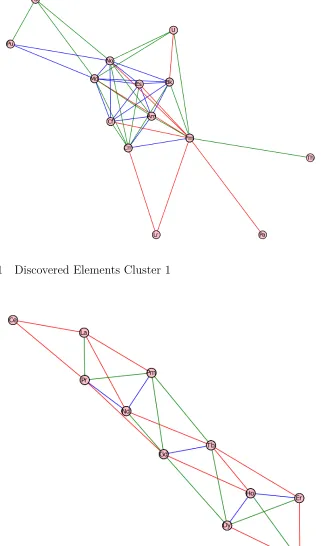
gen-erated connection matrix would.The figures shown below represent the strongest 3%
of the connections found, ignoring all of the weaker connections. It is important to
3% of all connections. For example, one cluster shows nickel, iron and cobalt all
con-nected. Since these connections appear above the threshold, they are in the strongest
3% of all of the connections found in the analysis. The range of connection values in
that top 3% was evenly divided into 3 parts and the connection between nickel and
cobalt falls into that top group, and thus is colored blue. The other two connections
fall into the second strongest group of the top 3% and are thus colored green.
The clusters picked out by this analysis are closely associated with each other on
the periodic table. In this case, only physical properties of the elements were used.
Figure 5.1 Discovered Elements Cluster 1
Chapter 6
Conclusion
The three methods of analysis described here offer three new ways of looking at
networks and how those networks can be classified and better understood. By
mod-eling networks as imaginary flows and using the connection matrix to generate a
Markov monoid, several analysis problems were overcome. From expanding unknown
networks in terms of known network types to finding clusters using eigenvalues /
eigenvectors and node properties, the tools developed for this study can be used to
study any type of network.
In this work, three hypotheses of Johnson’s were tested by writing the software
and performing the analysis on sample networks. First, the comparison of networks
using multi-order Renyi entropy curves was implemented. This allowed for the
"dis-tance" from unknown networks to known networks to be calculated regardless of
the relative sizes of the networks. An expansion of any network in terms of known
standard network types is possible. This same software allows for the comparison
of one network at different points in time to see how the network evolves. Second,
the idea that clusters could be detected by studying the eigenvalues and eigenvectors
of the resulting M matrix was tested and shown to be valid. The result was that
the eigenvalues showed the relative strengths of the clusters, and the elements of the
eigenvectors pointed out the nodes that were included in the clusters. Finally, the
idea that a table of properties and entities could be used to generate a connection
matrix was tested. In the table of elements, for example, the algorithm revealed
network analysis was possible only after linking the network to the Markov monoid
so that traditional matrix operations could be used.
The programs built for this project and used to analyze the data described here
were written in Sage and were written to analyze networks represented by text files in
a very general format. The goal is to allow any network to be easily converted into a
form which can be analyzed using these three tools. Work on new applications based
on this research is already underway with the goal to detect network anomalies that
could indicate network intrusion. The software can be easily modified to analyze any
type of data, however, by simply writing pre-processing routines for any dataset that
puts the data in the format required by the main software routines. The analysis can
then proceed completely independent of the type of network being analyzed. The
analysis engines are general purpose, and the future uses offer many areas for other
Bibliography
[1] Joseph E. JohnsonMarkov-type Lie Groups in GL(n,R) Journal of Mathematical
Physics Volume 26, No. 2, February 1985, pp. 252-257.
[2] Joseph E. JohnsonNew Advances for the Analysis and Tracking of Networks2006.
[3] Joseph E. Johnson Networks, Markov Lie Monoids, And Generalization Entropy,
St. Petersburg Russia Complexity Conference, March 2005
[4] Joseph E. JohnsonMarkov Lie Monoid Entropies as Network Metrics May 2006
[5] Joseph E. Johnson, personal communication
[6] Vladimir Estivill-Castro Why So Many Clustering Algorithms - A Position Paper
ACM SIGKDD Explorations Newsletter 4, June 2002, pp.65-75
[7] Ines Färber, Stephan Günnemann, Hans-Peter Kriegel, Peer Kröger, Emmanuel
Müller, Erich Schubert, Thomas Seidl, Arthur Zimek On Using Class-Labels in
Evaluation of Clusterings, 2010
[8] Emily Singer In Natural Networks, Strength in Loops Quanta Magazine, August
2013
[9] Brona McVittie Networks in NatureApoNET, 2010
[10] Amir Bashan, Yehiel Berezin, Sergey V. Buldyrev, Shlomo HavlinThe Extreme
Vulnerability of Interdependent Spatially Embedded Networks Nature Physics 9,
August 25, 2013, pp 667-672
[11] Sitabhra SinhaPhysics of Complex NetworksProceedings of the DAE Solid State Physics Symposium (2007)
[12] Brett Meador A Survey of Computer Network Topology and Analysis Examples
[13] Gilbert Strang Linear Algebra And Its Applications copyright 1988, Harcourt Brace Jovanovich, Inc., pp. 266-269
[14] Alfréd RényiOn Measures of Entropy and Information, Proceedings of the fourth Berkeley Symposium on Mathematics, Statistics and Probability 1960. pp. 547-561
[15] J. Chandrakanta Badajena, Chinmayee Rout Incorporating Hidden Markov
Model into Anomaly Detection Technique for Network Intrusion Detection,
In-ternational Journal of Computer Applications, Vol. 53, No. 11, September 2012, pp. 42-47
[16] S. Bridasri, K Saravanan Survey of Network Anomaly Detection Using Markov
Chain International Journal of Computer Science, Engineering and Information
Technology, Vol. 4, No. 1, February 2014, pp. 49-55
[17] Suratna BudalakotiAnomaly Detection Using Hierarchical Hidden Markov
Mod-els University of California Santa Cruz
[18] Christian Callagari Statistical Approaches for Network Anomaly Detection
ICIMP Conference, May 9 2009
[19] J. Diaz-Verdejo, G. Macia-Fernandez, P. Garcia-Teodoro, J. Nuno-Garcia
Anomaly Detection in P2P Networks Using Markov Modelling2009 First
Interna-tional Conference on Advances in P2P Systems, pp. 156-159
[20] Rafiul Hassan, Baikunth Nath, Michael Kirley A Data Clustering Algorithm
Based On Single Hidden Markov Model Proceedings of the International
Multi-conference on Computer Science and Information Technology, 2006, pp. 57-66
[21] Santo Fortunato Community Detection In Graphs Complex Networks and
Sys-tems Lagrange Laboratory, January 2010
[22] M. Girvan, M. E. J. Newman Community Structure In Social And Biological
Networks PNAS, Vol. 99, No. 12, June 11 2002, pp. 7821-7826
[23] Farnaz Moradi, Tomas Olovsson, Phillippas Tsigas An Evaluation Of
Commu-nity Detection Algorithms On Large-Scale Email Traffic Computer Science and
Technology ,Chalmers University of Technology
[24] Joseph E. Johnson, John W. Campbell Using the ExaSphere Network Analysis