International Journal in Management and Social Science
http://www.ijmr.net
147
CONSTRUCTION OF MIXED SAMPLING PLANS
INDEXED THROUGH MAPD AND IQL WITH LINK
SAMPLING PLAN AS ATTRIBUTE PLAN USING
WEIGHTED POISSON DISTRIBUTION
*R. Sampath Kumar
**R. Kiruthika
**R. Radhakrishnan
ABSTRACT
This paper presents the procedure for the construction and selection of mixed sampling plan
with MAPD as a quality standard and link sampling plan as attribute plan using weighted
Poisson distribution as a base line distribution. The plans are constructed indexed through
MAPD and IQL and also compared. Tables are constructed for the easy selection of the
plans.
Keywords and Phrases: Maximum allowable percent defective, Indifference quality level,
Operating characteristic, Tangent intercept.
AMS (2000) Subject Classification Number: Primary: 62P30 Secondary: 62D05
* Assistant Professor, Department of Statistics, Government Arts College, Coimbatore.
** Assistant Professor in Statistics, Kalaignar Karunanidhi Institute of Technology, Coimbatore.
International Journal in Management and Social Science
http://www.ijmr.net
148
1. INTRODUCTION
Mixed sampling plans consist of two stages of rather different nature. During the first stage
the given lot is considered as a sample from the respective production process and a criterion
by variables is used to check process quality. If process quality is judged to be sufficiently
good, the lot is accepted. Otherwise the second stage of the sampling plan is entered and lot
quality is checked directly by means of an attribute sampling plan.
There are two types of mixed sampling plans called independent and dependent plans. If the
first stage sample results are not utilized in the second stage, then the plan is said to be
independent otherwise dependent. The principal advantage of a mixed sampling plan over
pure attribute sampling plans is a reduction in sample size for a similar amount of protection.
It is the usual practice that while selecting a sampling inspection plan, to fix the operating
characteristic (OC) curve in accordance with the desired degree of discrimination. The
sampling plan is in turn fixed through suitably chosen parameters. The entry parameters used
in the acceptance sampling literature are acceptable quality level (AQL), indifference quality
level (IQL), limiting quality level (LQL) and maximum allowable percent defective (MAPD).
Several authors have provided procedures to design the sampling plans indexed through these
parameters for various acceptance sampling plans.
The concept of MAPD ( p*) was introduced by Mayer (1967) and further studied by
Soundararajan (1975) is the quality level corresponding to the inflection point on the OC
curve. The degree of sharpness of inspection about this quality level ‘ p*’ is measured
through ‘pt’, the point at which the tangent to the OC curve at the inflection point cuts the
proportion defective axis. One of the desired properties of an OC curve is that the decrease of
) (p
Pa should be slower for lesser values of ‘p’ and faster for greater values of ‘p’. If we set
*
p as the quality standard, the above property of the OC curve is obtained since p*
corresponds to the inflection point of the OC curve and hence
2 2
/ ) (p dp P
d a = 0 for p=p*
2 2P (p)/dp
International Journal in Management and Social Science
http://www.ijmr.net
149
2 2
/ ) (p dp P
d a > 0 for p>p*
The mixed sampling plan has been designed under two cases of significant interest. In the
first case sample size n1 is fixed and a point on the OC curve is given. In the second case
plans are designed when two points on the OC curve are given. The procedure for designing
the mixed sampling plans to satisfy the above mentioned conditions was provided by
Schilling (1967). Using Schilling’s procedure, Devaarul (2003) has constructed tables for
mixed sampling plans (independent case) having various sampling plans as attribute plans.
Link sampling plan comes under conditional sampling plans, which is classified as
cumulative type of sampling plan. The Conditional sampling procedures have been developed
to reduce the sample size and the inspection cost of the decision process using sample results
from neighboring ad related lots. This is the main advantage of conditional sampling plans.
But, when the process quality slowly changes the sample results from the past lots do not
reveal the exact situation. Harishchandra and Srivenkataramana (1982) have developed link
sampling plans. Sampath Kumar et.al (2012) and Radhakrishnan et.al (2010) have made
contributions to mixed sampling plan for independent case. Sampath Kumar (2007) has
constructed mixed sampling plan with various sampling plans as attribute plans using Poisson
distribution as a base line distribution.
The weighted Poisson distribution plays an important role in the acceptance sampling, mainly
in the construction of sampling plans. Each outcome (number of defectives) is specific but
can be assigned with different weights based on its importance or usage. In using weighted
Poisson distribution with weights Xα, α =1 the range of the distribution curtailed to 1, 2, 3…
from 0, 1, 2… This distribution can be viewed as a truncated Poisson distribution truncated at
x =0. It will be more useful to the industries which concentrates on second’s quality lots and
also to the industries which has atleast one defective in the majority of the manufacturing
lots. Even though the modern technologies aim at zero defective/ defects but practically it is
very difficult to make the lot as zero defective lot. In this context, the application of weighted
Poisson distribution in the construction of sampling plans is very relevant and it has many
features /advantages also.
Radhakrishna Rao(1977) suggested a weighted Binomial distribution can be used in
International Journal in Management and Social Science
http://www.ijmr.net
150 weighted Poisson distribution as a base line distribution. Mohana Priya (2008), Sampath
Kumar et.al (2011), Radhakrishnan and Mohana Priya (2008 a, 2008 b) have constructed the
sampling plans using weighted Poisson distribution as a base line distribution.
In this paper, mixed sampling plan (independent case) with link sampling plan as attribute
plan is constructed using weighted Poisson distribution as a base line distribution. The plans
indexed through MAPD and IQL are constructed separately by fixing the values of c1, c2 and
βj'. The mixed plans indexed through MAPD and IQL are also compared.
2. GLOSSARY OF SYMBOLS
The symbols used in this paper are as follows:
p : submitted quality of lot or process
Pa (p) : probability of acceptance for given quality p
p* : maximum allowable percent defective
pt : the point at which the inflection tangent of the OC curve cuts the ‘p’ axis
p0 : the submitted quality level such that Pa (p0) = 0.50
h* : relative slope at p*
n1 : sample size for the variable sampling plan
n2 : sample size for the attribute sampling plan
c1 : first attributes acceptance number
c2 : second attributes acceptance number
c3 : third attributes acceptance number
d : number of defectives in the sample
βj : probability of acceptance for lot quality ‘pj’
βj' : probability of acceptance assigned to first stage for percent defective p j
βj'' : probability of acceptance assigned to second stage for percent defective pj
International Journal in Management and Social Science
http://www.ijmr.net
151
3. OPERATING PROCEDURE OF MIXED SAMPLING PLAN HAVING LINK SAMPLING PLAN AS ATTRIBUTE PLAN
Schilling (1967) has given the following procedure for the independent mixed sampling
plan with upper specification limit (U) and standard deviation (σ).
1. Determine the parameters of the mixed sampling plan n1, n2, k, c1, c2 and c3.
2. Take a random sample of size n1 from the lot.
3. If a sample average X ≤ A = U- k
, accept the lot4. If the sample average X > A = U- k , take another sample of size n2 from the lot ‘i’ ad
count the number of defectives di there i.
5. If the number of defectives di ≤ c1, accept the lot.
6. If the number of defectives di < c3, reject the lot.
7. If c1 < Di ≤ c3, combine the total number of defectives from the immediate part and future
lots, Di=di-1+di+di+1
8. If Di ≤ c2, accept the lot ‘i’ and reject the lot if Di>c3
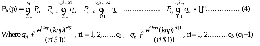
The OC function of the mixed sampling plan, suggested by Schilling (1967) for single
sampling plan is
) 1 .( ... ... ... ... ... ... ... ... )... ; ( ) ( ) ( ) ( 2 0 1
1 x A P x A P jn
P p P c j n n a
Equation (1) can be expressed as βj = βj'+ (1- βj') βj''.
By taking the link sampling plan as attribute plan, equation (1) can be written as
) 2 .( ... . ... ... ) ( ) ( ) ( 2 1 1 2 1 1 1 1 1
3 3 2
2 1 1 3 1 1 1
c c i c c i ri c ri c c c i ri c c i ri n na p P x A P x A P P q P q P q
P i Where )! 1 ( ) ( 1 ri np e P ri np
ri , ri = 1,2,……c2
)! 1 ( ) ( 1 ri knp e q ri knp
ri , ri= 1,2………c3-(c1+1)
International Journal in Management and Social Science
http://www.ijmr.net
152
4. CONSTRUCTION OF MIXED SAMPLING PLAN HAVING LINK SAMPLING PLAN AS ATTRIBUTE PLAN USING WEIGHTED POISSON DISTRIBUTION
The detailed procedure adopted in this paper for the construction of mixed sampling plan
having link sampling as attribute plan using weighted Poisson distribution indexed through
MAPD is given below:
Assume that the mixed plan is independent
Decide the sample size n1 (for variable sampling plan) to be used.
Calculate the acceptance limit for the variable sampling plan as
* * )/ 1
' ( { ) (
[z p z n U
A }]
, where z is standard normal variate correspondingto‘t’ such that t = e du t z u
) ( 2 2 2 1 Split the probability of acceptance β* as β*' and β*''such that β* =β*' + (1- β*') β*''. Fix the
value of β*' .
Determine β*'', the probability of acceptance assigned to the attribute plan associated with
the second stage sample as β*''= (β* - β*')/ (1- β*').
Determine the appropriate second stage sample of n2 from the relation
β*'' =
2 1 1 2 1 1 1 1 13 3 2
2 1 1 3 1 . ... ... c c i c c i ri c ri c c c i ri c c i
ri P q P q P q
P i Where )! 1 ( ) ( 1 ri np e P ri np
ri , ri = 1, 2,……c2
)! 1 ( ) ( 1 ri knp e q ri knp
ri , ri= 1, 2………c3-(c1+1)
Using the above procedure, tables have been constructed to facilitate easy selection of mixed
sampling plan using link sampling plan as attribute plans indexed through MAPD.
4.1 CONSTRUCTION OF TABLES
The OC function of weighted Poisson distribution for single sampling plan is given
International Journal in Management and Social Science
http://www.ijmr.net
153
0 ) ; ( ) , ( ) ( x a x p x x p x p P ; x=0, 1, 2…………. .………
(3)
The probability of acceptance for link sampling plan under weighted Poisson
distribution when α = 1 is used in this paper for determining the second stage probabilities
and is given by
Pa (p) =
2 1 1 2 1 1 1 1 1
3 3 2
2 1 1 3 1 . ... ... c c i c c i ri c ri c c c i ri c c i
ri P q P q P q
P
i = βj''……… (4)
Where )! 1 ( ) ( 1 ri knp e q ri knp
ri , ri = 1, 2,……c2 ,
)! 1 ( ) ( 1 ri knp e q ri knp
ri , ri= 1, 2………c3-(c1+1)
Using the equation (4) the inflection point (p*) is obtained by using 0
) ( 2 2 dp p p d a and 0 ) ( 3 3 dp p p d a .
The relative slope of the OC curve h* is given by, h* =
( ) ( ) a a dP p p
P p dp
at p=p*.
The inflection tangent of the OC curve cuts the ‘p’ axis at pt =p* + (p*/h*). The
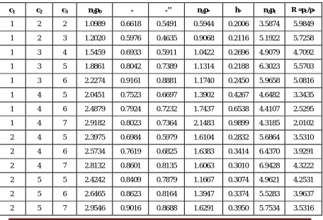
values of n2p*, h*, n2pt and R= pt / p* are calculated for the specified β*' = 0.25 using C
program and presented in Table 1.
4.2 SELECTION OF THE PLAN
Table 1 is used to construct the plans when MAPD (p*) and tangent intercept (pt) are given.
For any given values of c1, c2, pt and p* one can find the ratio R = pt / p*. Corresponding to
the value of c1 and c2 find the value in Table1 under the column R which is equal to or just
greater than the specified ratio, the corresponding value of c3 is noted. From this c1,c2 and c3
values one can determine the value of ‘n’ using n2 = n2 p*/ p*.
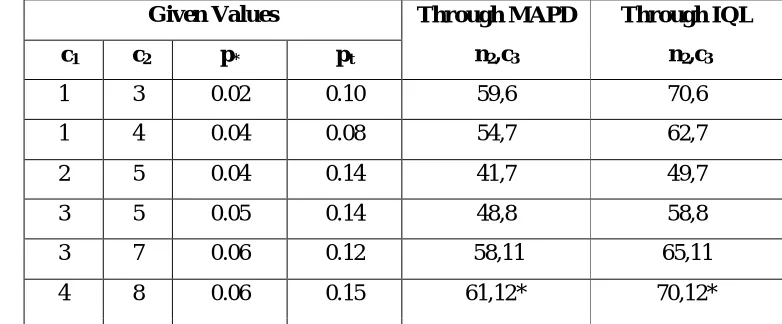
Example 1: Given c1 = 4, c2 = 8, p* = 0.06, pt =0.15and β*' = 0.25. Find the ratio R= pt /p* =
2.5. Using Table 1, corresponding to c1 = 4, c2=8 select the value of R equal to or just greater
International Journal in Management and Social Science
http://www.ijmr.net
154 (3.6448/0.06) = 61. The Mixed Sampling plan with link sampling plan as attribute plan is,
n2=61, c1 = 4, c2=8 and c3=12 and the OC curve is presented in Figure1.
5. SELECTION OF MIXED SAMPLING PLAN HAVING LINK SAMPLING PLAN
AS ATTRIBUTE PLAN INDEXED THROUGH IQL
The general procedure given in section 4 is used for designing the mixed sampling plan
having link sampling plan as attribute plan indexed through IQL (p0). For the specified values
of β0=0.50 and β0' =0.25, the n2p0 values are calculated for different values of c1, c2 and c3
using C program and presented in Table1.
5.1 SELECTION OF THE PLAN
Table 1 is used to construct the plans when IQL (p0), c1, c2, c3
values
are given. For anyspecified values of p0, c1 ,c2 and c3 one can determine n2 value using n2= n2p0 / p0.
Example 2: Given po= 0.07, c1 = 4, c2 = 7, c3
= 11
and β0' =0.25. Using Table 1, find n2=n2p0/p0= 4.8788/0.07=70. For a fixed β0' =0.25, the mixed sampling plan with link sampling
plan as attribute plan is n2= 70, c1= 4, c2=7 and c3=11.
6. COMPARISON OF PLANS INDEXED THROUGH MAPD AND IQL
In this section the mixed sampling plan with link sampling plan as attribute plan indexed
through MAPD is compared with the mixed sampling plan with link sampling plan as
attribute plan indexed through IQL by fixing the parameters c1,c2 and β0'.
For the specified values of p* and pt with the assumption β*' = 0.25 one can find the values of
c3 and n2 indexed through MAPD as in section 4. By fixing the values of c1, c2 and n2, find
the value of p1 by equating Pa (p) = β0= 0.50. Using β0' =0.25 ,c1, c2 and p0 one can find the
value of n2 using n2 = n2p0/p0 from Table 1. For different combinations of c1,c2, p* and pt, the
values of n2, c3(indexed through MAPD) and n2, c3 (indexed through IQL) are calculated and
International Journal in Management and Social Science
http://www.ijmr.net
155
Table 2: Comparison of plans
Given Values Through MAPD
n2,c3
Through IQL
n2,c3
c1 c2 p* pt
1 3 0.02 0.10 59,6 70,6
1 4 0.04 0.08 54,7 62,7
2 5 0.04 0.14 41,7 49,7
3 5 0.05 0.14 48,8 58,8
3 7 0.06 0.12 58,11 65,11
4 8 0.06 0.15 61,12* 70,12*
* OC Curves are drawn
7. CONCLUSION
In this paper the procedure for constructing mixed sampling plans with link sampling plan
attribute plan indexed through MAPD and IQL with weighted Poisson distribution as the
baseline distribution are presented. Suitable tables are also provided for the easy selection of
the plans for the engineers who are working on the floor of the assembly. It is concluded
from the study that the second sample size required for mixed sampling plan with link
sampling plan as attribute plan indexed through MAPD is less than that of the second stage
0 0.1 0.2 0.3 0.4 0.5 0.6 0.7 0.8 0.9 1
0 0.02 0.04 0.06 0.08 0.1 0.12 0.14
P
ro
b
a
b
il
it
y
o
f
a
c
c
e
p
ta
n
c
e
Product quality in proportion defectives
Figure 1: OC Curves for LSP with n=61 (MAPD),
n=70 (IQL) , c1=4, c2= 8, c3= 12
International Journal in Management and Social Science
http://www.ijmr.net
156 sample size of the mixed sampling plan with link sampling plan as attribute plan indexed
through IQL, justified by Sampath Kumar (2008). These plans definitely help the producers,
because of the lesser sample size which directly result in lesser sampling cost and indirectly
reduces the total cost of the product. The different sampling plans can also be constructed
by changing the first stage probabilities (β*' and β0') and can be compared for their
efficiency.
REFERENCES
1. Devaarul, S (2003). ‘Certain Studies Relating to Mixed Sampling Plans and Reliability based Sampling Plans’, Ph.D., Dissertation, Department of Statistics, Bharathiar University, Coimbatore, Tamil Nadu, India.
2. Harishchandra, K. and Srivenkataramana, T. (1982). ‘Link sampling for attributes’, Communications in Statistics, ‘Theory and Methods’, Vol.11, No.16, pp.1855-1868.
3. Mayer, P.L. (1967). ‘A note on sum of Poisson probabilities and an application’, ‘Industrial Quality Control’, Vol.19, No.5, pp.12-15.
4. Mohana Priya, L. (2008). ‘Construction and Selection of Acceptance Sampling Plans based on Weighted Poisson Distribution’, Ph.D., Dissertation, Department of Statistics, Bharathiar University, Coimbatore, Tamil Nadu, India.
5. Radhakrishna Rao, C. (1977). ‘A natural example of a weighted binomial distribution’, The American Statistician, Vol.31, No.1
6. Radhakrishnan, R. and Mohana Priya, L.(2008 a). ‘Selection of single sampling plan using conditional weighted Poisson distribution’, ‘International Journal of Statistics and Systems’, Vol.3, No.1, pp. 91-98.
7. Radhakrishnan, R. and Mohana Priya, L. (2008 b). ‘Comparison of CRGS plans using Poisson and weighted Poisson distribution’, ‘Probstat Forum’, Vol.1, No.1, pp.50-61.
8. Radhakrishnan, R. Sampath Kumar, R. and Malathi, M. (2010). ‘Selection of mixed sampling plan with TNT- (n1, n2; 0) plan as attribute plan indexed through MAPD and
MAAOQ’, ‘International Journal of Statistics and system’, Vol.5, No.4, pp.477-484.
9. Sampath Kumar, R. (2007). ‘Construction and Selection of Mixed Variables-Attributes Sampling Plans’ - Ph.D., Dissertation, Department of Statistics, Bharathiar University, Coimbatore, Tamil Nadu, India.
10.Sampath Kumar, R. Kiruthika, R. and Radhakrishnan, R. (2011). ‘Comparison of mixed sampling plan indexed through MAPD and LQL with single sampling plan as attribute plan using weighted Poisson distribution’, ‘Journal of statistics science’, Vol.3, No.2,pp. 165-173.
International Journal in Management and Social Science
http://www.ijmr.net
157 through MAPD and AQL using intervened random effect Poisson distribution’, ‘Global journal of Management science and technology’, Vol.1, No. 4.
12.Schilling, E.G (1967). ‘A General Method for Determining the Operating Characteristics of Mixed Variables’-‘Attributes sampling plans Single side specifications, S.D.known’, Ph.D., Dissertation- Rutgers- The State University, New Brunswick, New Jersy.
13.Soundararajan, V. (1975). ‘Maximum allowable percent defective (MAPD) single sampling inspection by attribute plan’, ‘Journal of Quality Technology’, Vol.7, No.4, pp.173-182.
14. Subramani, K .(1991). ‘Studies on Designing Attribute Acceptance Sampling Plans with Emphasis on Chain Sampling plans’, Ph.D Thesis, Bharathiar University, Coimbatore, Tamil Nadu, India.
15. Sudeswari (2002). ‘Designing of Sampling Plan using Weighted Poisson distribution. M.Phil., Dissertation, Department of Statistics, PSG College of Arts and Science, Coimbatore.
Table 1: Various characteristics of the mixed sampling plan when (p*, β*) and (p0, β0) are
known for a specified β*' = 0.25, β0=0.50 and β0' =0.25
c1 c2 c3 n2p0 β* β*'' n2p* h* n2pt R =pt /p*
1 2 2 1.0989 0.6618 0.5491 0.5944 0.2006 3.5874 5.9849
1 2 3 1.2020 0.5976 0.4635 0.9068 0.2116 5.1922 5.7258
1 3 4 1.5459 0.6933 0.5911 1.0422 0.2696 4.9079 4.7092
1 3 5 1.8861 0.8042 0.7389 1.1314 0.2188 6.3023 5.5703
1 3 6 2.2274 0.9161 0.8881 1.1740 0.2450 5.9658 5.0816
1 4 5 2.0451 0.7523 0.6697 1.3902 0.4267 4.6482 3.3435
1 4 6 2.4879 0.7924 0.7232 1.7437 0.6538 4.4107 2.5295
1 4 7 2.9182 0.8023 0.7364 2.1483 0.9899 4.3185 2.0102
2 4 5 2.3975 0.6984 0.5979 1.6104 0.2832 5.6864 3.5310
2 4 6 2.5734 0.7619 0.6825 1.6383 0.3414 6.4370 3.9291
2 4 7 2.8132 0.8601 0.8135 1.6063 0.3010 6.9428 4.3222
2 5 5 2.4242 0.8409 0.7879 1.1667 0.3074 4.9621 4.2531
2 5 6 2.6465 0.8623 0.8164 1.3947 0.3374 5.5283 3.9637
International Journal in Management and Social Science
http://www.ijmr.net
158
2 5 8 3.3108 0.9230 0.8973 1.9697 0.3601 7.4355 3.7749
3 5 8 3.6153 0.7869 0.7159 2.3840 0.3533 7.1011 2.9786
3 5 9 3.7841 0.8768 0.8357 2.1789 0.3192 9.0050 4.1328
3 6 8 3.6962 0.7788 0.7051 2.4299 0.3666 9.0581 3.7278
3 6 9 3.9011 0.7963 0.7284 2.6705 0.4991 8.0211 3.0036
3 7 8 3.7115 0.7799 0.7065 2.4610 0.3719 9.0784 3.6889
3 7 9 3.9713 0.8037 0.7383 2.7154 0.4960 8.1899 3.0161
3 7 10 4.3102 0.8227 0.7636 3.0587 0.6999 7.4288 2.4287
3 7 11 4.6764 0.8345 0.7793 3.4498 0.9661 7.0207 2.0351
4 7 11 4.8788 0.9570 0.9427 2.5273 0.3456 9.8400 3.8934
4 7 12 5.0991 0.8191 0.7588 3.6097 0.6546 9.1241 2.5277
4 8 11 4.9386 0.8241 0.7655 3.3503 0.5679 9.2498 2.7608
4 8 12 5.1995 0.8406 0.7875 3.6448 0.6158 9.5636 2.6239