International Journal in IT and Engineering, Impact Factor- 4.747
ABSTRACT
Global Positioning System (GPS) is a satellite based navigation system designed to provide instantaneous Position, Velocity and Time (PVT) information almost anywhere on the globe at any time and in all weather conditions. Using the GPS one can determine his exact location (latitude, longitude, altitude) in ECEF coordinates accurate to within a range of 20m to approx. 1mm. User can also determine the time accurately to within a range of 60ns to approx. 5ns.
The user estimates an apparent or pseudo range to each SV (Satellite Vehicle) by measuring the transit time of the signal. The pseudo range ‘’, is a biased and noisy measurement of the true range. The signal coming from a GPS satellite will be contaminated by various errors like ephemeris error, propagation error in the form of ionospheric and tropospheric delays, satellite and receiver clock biases with respect to GPS Time (GPST), multipath error etc. The accuracy with which we can measure the true range ‘r’ depends upon our ability to compensate for the biases and errors. This paper describes methods of determining various errors such as ionospheric delay, troposheric delay and the satellite clock bias to determine the true range from each satellite and finally the receiver position (xu, yu. zu) is obtained by using linearization technique. The results compared with the exact values measured by the receiver are found to be accurate.
Keywords: GPS, GPST, Pseudo range, RINEX, SV
I.INTRODUCTION
A GPS user estimates an apparent or pseudo range to each SV (Satellite Vehicle) by measuring the transit time of the signal. Using the pseudo ranges, user position in 3-D (latitude, longitude and height) and the time offset between the transmitter and receiver clock can be estimated after making appropriate corrections for the observed pseudoranges. If the unknown coordinates of the user position are represented by xu, yu and zu and
the known positions of Satellite Vehicles are with xj, yj, zj, (where j = 1,2,3,4) in ECEF coordinate system, the
user position (in 3-D) and time offset ‘tu‘ are obtained by simultaneously solving the nonlinear equations given
below.
The measured pseudo range from each satellite is given by
= r + c[tu - ts] + I + T+ (1)
Where ‘c’ is the free space velocity of electromagnetic signals I = Ionospheric delay
I = Tropospheric delay
tu = Receiver clock bias with respect to GPS Time
ts = Satellite clock bias with respect to GPS Time
LINEARIZATION TECHNIQUE FOR MEASUREMENT OF GPS USER POSITION
Prof B.HARI KUMAR1, B.ARCHANA2, G.MANASA3, CH.MUVVA KRISHNA KUMAR4
1. Prof. & Head, ECE Department, BRINDAVAN INSTITUTE OF TECHNOLOGY & SCIENCE, KURNOOL, AP, INDIA.
2. Senior U.G Student, BRINDAVAN INSTITUTE OF TECHNOLOGY & SCIENCE, KURNOOL, AP, INDIA.
3. Senior U.G Student, BRINDAVAN INSTITUTE OF TECHNOLOGY & SCIENCE, KURNOOL, AP, INDIA.
= Un-modeled errors
The true range ‘r’ from each satellite is given by
2 22
u j u
j u
j
j x x y y z z
; j =1, 2, 3, 4 (2)
The ranges measured from satellites are called pseudo ranges since biases in the receiver clock prevent the precise measurement of true ranges. To determine the receiver position accurately, all the errors have to be estimated and compensated for. In this paper, the ionospheric delay is estimated using Klobuchar model [3]. Hopfield model is used for the estimation of tropospheric delay.
Ionospheric delay. Tropospheric delay, Satellite clock bias and the Relativistic effects have been estimated and corrections have been made to estimate the true ranges. Using the corrected ranges position of the user in ECEF coordinates is estimated using ‘Linearization Technique’.
II.GPSERRORS a) Satellite Clock Error:
Although all the satellites carry atomic clocks that are very accurate, these can deviate from GPS system time (GPST), which results in pseudo range error. GPS Time (GPST) is a composite time scale derived from the times kept by clocks at GPS monitor stations and aboard the satellites and is used as the reference time. Ranging errors induced by clock errors are of the order of 3.0m. The Master Control Station determines the clock error of each satellite and transmits clock correction parameters to the satellites for rebroadcast of these in the navigation message. The receiver using these parameters implements necessary corrections.
The SV clock correction for the C/A code pseudo range is given by:
ts=af
0 + af1 * (t - toc) + af2 * (t - toc)2 + tr (3)
af0 = clock bias (sec)
af1 = clock drift (sec/sec)
af2 = frequency drift (sec/sec2)
toc = clock data reference time (sec)
t = current time epoch (sec)
tr = correction due to relativistic effects (sec)
b) Relativistic Effects:
Both general and special theories of relativity affect the satellite clock. Need for general relativistic corrections arise when the signal source (satellite) and signal receiver (GPS receiver) are located at different gravitational potentials. Special relativity relativistic corrections arise any time the signal source or the signal receiver is moving with respect to the chosen isotropic frame, which in the GPS system is the ECI frame. In order to compensate for both of these effects, the satellite clock frequency is adjusted to 10.22999999545 MHz prior to launch. The frequency observed by the user at sea level would be 10.23 MHz, hence the user does not have to correct for this effect.
But the user has to make a correction for another relativistic effect that arises because of the slight eccentricity of the satellite orbit. When the satellite is at perigee, the satellite velocity is higher and the gravitational potential is lower because of which the satellite clocks run slower. When the satellite is at apogee, the satellite velocity is lower and the gravitational potential is higher and the satellite clocks run faster. This effect can be compensated as follows
tr= Fe a SinEk (4)
Where
International Journal in IT and Engineering, Impact Factor- 4.747
a = semi-major axis of the satellite orbitEk = eccentric anomaly of the satellite orbit
Due to rotation of the Earth during the time of signal transmission, a relativistic error is introduced which is called the sagnac effect. During the propagation time of the SV signal transmission, a clock on the surface of the earth will experience a finite rotation with respect to the resting reference frame at the geocenter. If the user experiences a net rotation away from SV, the propagation time will increase and vice versa
c) Atmospheric Errors
The satellite signals propagate through atmospheric layers as they travel from the satellite to the receiver. Two layers are generally considered when dealing with GPS: the Ionosphere, which extends from a height of 70 to 1000 km above the Earth, and the Troposphere which stretches to about 16 kms. above the equator and 9 kms. above the poles from the surface of the earth.
As the signal propagates through the ionosphere, the carrier experiences a phase advance and the codes experience a group delay. In other words, the GPS code information is delayed resulting in the pseudo ranges being measured too long as compared to the geometric distance to the satellite. The extent to which the measurements are delayed depends on the Total Electron Content (TEC) along the signal path, which is a measure of the electron density. Further this is dependent on three factors: the geomagnetic latitude of the receiver, the time of day and the elevation of the satellite. Significantly larger delays occur for signals emitted from low elevation satellites (since they travel through a greater section of the ionosphere), peaking during the daytime and subsiding during the night (due to solar radiation). In regions near the geomagnetic equator or near the poles, the delays are also larger.
The ionospheric delay is frequency dependent and can therefore be eliminated using dual frequency GPS observations; hence the two carrier frequencies in the GPS design. Single frequency users, however, can partially model the effect of the ionosphere using the Klobuchar model. Eight parameters of this model are transmitted along with other navigation data from the satellites. These parameters depend on the time of day and the geomagnetic latitude of the receiver. The model results in an estimate of the vertical ionospheric delay, which is then combined with an obliquity factor, dependent on satellite elevation, producing a delay for the receiver-satellite line of sight. The final value provides an estimate within 50% of the true delay and produces delays ranging from 5m (night) to 30m (day) for low elevation satellites and 3-5m for high elevation satellites at mid latitudes.
The troposphere causes a delay in both the code and carrier observations. Since it is not frequency dependent (within the GPS L band range) it cannot be canceled out by using dual frequency measurements but it can, however, be successfully modeled. The troposphere is split into two parts: the dry component, which constitutes about 90% of the total refraction, and the wet part, which constitutes the remaining 10%. Values for temperature, pressure and relative humidity are required to model the vertical delay due to the wet and dry part, along with the satellite elevation angle, which is used with an obliquity/mapping function. Models put forward by Hopfield, Black and Saastamoninen are all successful in predicting the dry part delay to approximately 1-cm and the wet part to 5 cm. Ionospheric and tropospheric delays have been described in detail in the subsequent sections.
Ionospheric Delay:
The vertical time delay for the code measurement is given by
3
4
2
1 2
t A iono
v A
T
A
A Cos
(5)Where A1 = 5 nano seconds
2 3
2 1 2 3 4
m m m
IP IP IP
A
2 3
4 1 2 3 4
m m m
IP IP IP
A
The values for A1and A3 are constant, the coefficients i ,i , i = 1,2 --- 4 are uploaded to the satellites and broadcast to the user. The parameter ‘t’ in Eq. (5) is the local time of the ionospheric point IP and may be derived from
15
IP UT
t
t (6)Where IP is the geomagnetic longitude positive to east for the ionospheric point in degrees and tUT is the observation epoch in Universal Time. m
IP
is the spherical distance between the geomagnetic pole and the ionospheric point.Tropospheric Delay:
The tropospheric path delay is defined as
Tropn-1 ds
(7)In general, instead of the refractive index n the refractivity N is used. Where the refractivity
N
Trop
10 n-1
6
Equation becomes
Trop
10
-6
N
Tropds
(8) The tropospheric delay can be estimated using several models which are described below:Hopfield (1969) shows the possibility of separating NTrop into dry and wet components as Trop w Trop d Trop N N
N
(9)
Where the dry part results from the dry atmosphere and the wet part from the water vapor. Correspondingly the relations become
ds N 10-6 Tropd
Trop
d
andTropw 10-6NTropw ds
Trop w Trop
d Trop
10 N ds Trop d -6 Trop
d
+ 10-6 NTropw ds (10)
About 90% of the tropospheric refraction arise from the dry component and 10% from the wet component. There are a number of models which give us the dry and wet refractivity at the surface of the earth.
Dry component of refractivity is given by
1 -1 1 Trop o
d, , c 77.64 K mb
T p c
N (11)
Where p is the atmospheric pressure in millibar (mb) and T is the temperature in Kelvin (K). Wet component is given by 1 -2 5 3 1 -2 2 3 2 Trop o w, mb K 10 * 718 . 3 c and mb K 96 . 12 c , T e c T e c N (12)
Where e is the partial pressure of water vapor in mb.
According to Hopfield model the dry refractivity as a function of the height h above the surface is given by 4 d d Trop o d, Trop d h h h N h) ( N (13)
Where hd = 40136 +148.72 (T – 273.16) m. Substituting the above equation results in
ds h h h N 10 4 d d Trop o d, 6 Trop
d
International Journal in IT and Engineering, Impact Factor- 4.747
The integral can be solved if the delay is calculated along the vertical direction and if the curvature of the signal path is neglected. Thus, for an observation site on the surface of the earth (i..e., h=0), the above equation becomes
dh
d h
h 0 h 4 d 4 d Trop o d, 6 Tropd
(h
-
h)
h
1
N
10
(15)Where the constant denominator has been extracted. After integration,
|
0 5 4 d Trop o d, 6 Tropd
(
)
5
1
-h
1
N
10
h hdh d
h
h
(16)is obtained. The evaluation of the expression between the brackets gives 5 5 d h so that d
h
Trop o d, 6 Trop dN
5
10
(17)is the dry portion of the tropospheric zenith delay.
The wet portion is much more difficult to model because of the strong variations of the water vapor with respect to time and space. Nevertheless, due to the lack of an appropriate alternative, the Hopfield model assumes the same functional model for both the wet and dry components. Thus,
Trop w Trop
w
h
N
N
(
)
,04 w w h h h
; Where the mean value
h
w
11
,
000
m
(18)is used. Sometimes other values such as
h
w
12
,
000
m
have been proposed. Unique values forh
d andh
wcannot be given because of their dependence on location and temperature. The integration of above equation results in
w
h
Trop o w, 6 Trop wN
5
10
(19)Therefore, the total tropospheric zenith delay is
h
dh
w
Trop o w, Trop o d, 6 Trop
N
N
5
10
(20)With the dimension in meters. The model in its present form does not account for an arbitrary zenith angle of the signal. Considering the line of sight, an obliquity factor must be applied which, in its simplest form, is the projection from the zenith onto the line of sight. Frequently, the transition of the zenith delay to a delay with arbitrary zenith angle is denoted as the application of a mapping function.
Introducing the mapping function the above equation becomes
N
(
)
N
(
)
5
10
Trop o w, Trop o d, 6 TropE
m
h
E
m
h
d d
w w
(21)Where
m
d(E
)
andm
w(E
)
are the mapping functions for the dry and the wet part and E (expressed in degrees) indicates the elevation at the observing site (where the line of sight is simplified as straight line). Explicitly,)
(E
m
d =25
.
6
sin
1
2
E
(22))
(E
m
w =25
.
2
sin
1
2
E
(23)Trop
(E)= Trop d (E) + Trop w
(E) (24)
) ( Trop d E =
5
10
6)
11000
](
[
25
.
2
sin
)
10
(
718
.
3
96
.
12
2 2 5T
e
E
(25)Measuring p,T,e at the observation location and calculating the elevation angle E, the total tropospheric path delay is obtained in meters by the equations
III. LINEARIZATION TECHNIQUE
To determine the user position in three dimensions (xu, yu, zu) and the receiver clock offset tu, pseudoranges are
to be obtained from a minimum of four satellites.
u2 u j 2 u j 2 u j
j x x y y z z ct
ρ ; j = 1,2,3,4. (26)
The resulting equations can be written as a function of user coordinates and clock offset as
u u u u
j f x ,y ,z ,t
(27)Using an approximate position location (xˆu,yˆu,zˆu)and time bias estimate tˆu, an approximate pseudorange can
be calculated
j u
j u
j u
uj xˆ x yˆ y zˆ z ctˆ
ˆ 2 2 2
; j =1, 2, 3, 4
= f( xˆu, yˆu, zˆu, tˆu) (28)
The unknown user position and receiver clock offset are considered to consist of an approximate component and an incremental component as stated below.
u u
u x x
x ˆ
u u
u y y
y ˆ
u u
u z z
z ˆ u u
u t t
t ˆ
This allows writing Eq. (27) as f
xu,yu,zu,tu
f
xˆuxu,yˆuyu,zˆuzu,tˆu tu
This latter function can be expanded about the approximate point using a Taylor series. It can be shown that
u u j u j u j u j u j u j j
j z c t
r z z y r y y x r x x ˆ ˆ ˆ ˆ ˆ ˆ ˆ
Where rˆj
xˆjxu
2 yˆjyu
2 zˆjzu
2j j
j
ˆ j u j zj j u j yj j u j xj r z z a r y y a r x x a ˆ ˆ ; ˆ ˆ ; ˆ ˆ
Where axj, ayj and azj terms denote the direction cosines of the unit vector pointing from the approximate user position to the jth satellite.
Rewriting Equation (4.5) results into
j axjxu ayjyu azjzu ctu
When pseudorange measurements are made to four satellites (j = 4), Equation can be represented in matrix form as 4 3 2 1
x=
International Journal in IT and Engineering, Impact Factor- 4.747
1
1
1
1
4 4 4
3 3 3
2 2 2
1 1 1
z y x
z y x
z y x
z y x
a a a
a a a
a a a
a a a
H
We can obtain error matrix x from the following equation
1
H
x (29)
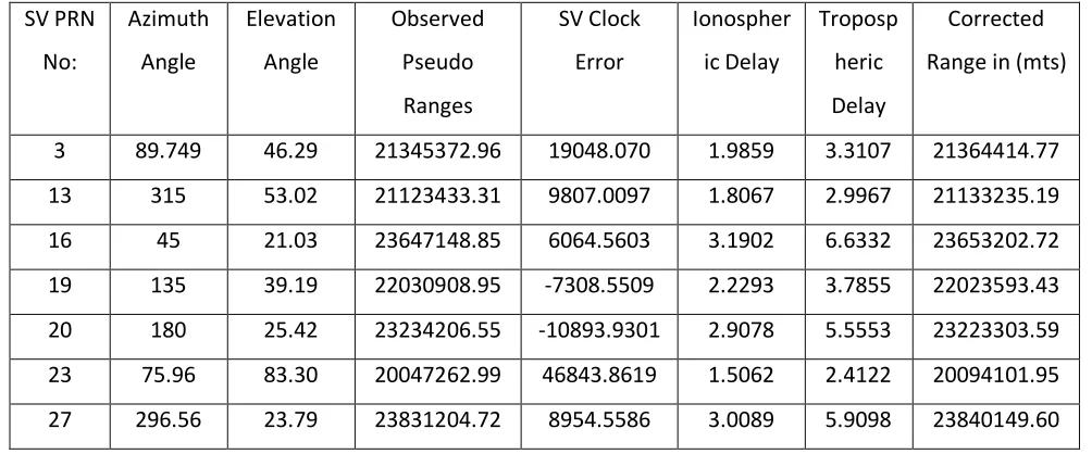
The above procedure is to be repeated till sufficient accuracy is obtained Table 1
Estimation of GPS Errors and Correction of Pseudo ranges
SV PRN
No:
Azimuth
Angle
Elevation
Angle
Observed
Pseudo
Ranges
SV Clock
Error
Ionospher
ic Delay
Troposp
heric
Delay
Corrected
Range in (mts)
3 89.749 46.29 21345372.96 19048.070 1.9859 3.3107 21364414.77
13 315 53.02 21123433.31 9807.0097 1.8067 2.9967 21133235.19
16 45 21.03 23647148.85 6064.5603 3.1902 6.6332 23653202.72
19 135 39.19 22030908.95 -7308.5509 2.2293 3.7855 22023593.43
20 180 25.42 23234206.55 -10893.9301 2.9078 5.5553 23223303.59
23 75.96 83.30 20047262.99 46843.8619 1.5062 2.4122 20094101.95
27 296.56 23.79 23831204.72 8954.5586 3.0089 5.9098 23840149.60
IV.RESULTSANDCONCLUSIONS
RINEX data from Chitrakut station (Near IIT Kanpur) is used for this purpose. The observation data of 3rd January
2006 at (0 hrs. 0 min. 0 sec) has been used. Seven satellites (SV PRN. Nos. 3 13 16 19 20 23 27) are observed at the epoch time. Algorithms have been implemented to sort out the ephemeris data into matrix format and for the determination of satellites’ position at the epoch time. By using clock correction parameters which are available as part of the Navigation message, the satellite clock bias and error due to relativistic effect have been obtained. The Ionospheric delay has been estimated using Kloubuchar model. All the eight coefficients for the implementation of Kloubuchar model are available as part of Navigation message. The Tropospheric delay has been estimated using Hopfield method. The estimated errors and the corrected ranges have been represented in Table 1. And finally the user position has been calculated using Linearization Technique and the results are indicated below.
Exact User Position in meters as per the observation data: Xu=918074.10, Yu=5703773.53, Zu =2693918.92
User position estimated using Linearization technique: Xu=918050.65, Yu=5703751.91, Zu=2693899.70
Results indicate that the estimated user position using linearization technique is agreeing with the exact position of the user as given in observation data. In order to further improve the accuracy in estimating the GPS user position, non-linear methods such as method of least squares can be used which requires additional circuitry for its implementation which increases the cost of the receiver.
REFERENCES
[1]. Bancroft. S, “An algebraic solution of the GPS equations”, IEEE Transactions on Aerospace and
Electronic Systems 21 (1985) 56–59.
[2]. B.HofmannWellenhof, .Lichtenegger and J.Collins, “GPS Theory and Practice”, Springer-Verlag
Wien, New York, 1992.
[3]. Klobuchar J, “Design and characteristics of the GPS ionospheric time – delay algorithm for single
frequency users”, Proceedings of PLANS’86, Las Vegas, Nevada, November 4-7, pp280-286.
[4]. Hopfield HS, “Two – quartic tropospheric refractivity profile for correcting satellite data”, Journal
of Geophysical research, 74(18): 4487-4499.
[5] Strang, G. and Borre, K., “Linear Algebra, Geodesy and GPS”, Wellesley Cambridge, Wellesley,
MA, 1997.
[6] http://home.iitk.ac.in/~ramesh/gps/
[7] Kaplan, E. D., "Understanding GPS: Principles and Applications", Artech House,1996.