An Optimal Medium Access Control with Partial
Observations for Sensor Networks
R ˘azvan Cristescu
Center for the Mathematics of Information, California Institute of Technology, Caltech 13693, Pasadena, CA 91125, USA Email:[email protected]
Sergio D. Servetto
School of Electrical and Computer Engineering, College of Engineering, Cornell University, 224 Philips Hall, Ithaca, NY 14853, USA Email: [email protected]
Received 10 December 2004; Revised 13 April 2005
We consider medium access control (MAC) in multihop sensor networks, where only partial information about the shared medium is available to the transmitter. We model our setting as a queuing problem in which the service rate of a queue is a function of a partially observed Markov chain representing the available bandwidth, and in which the arrivals are controlled based on the partial observations so as to keep the system in a desirable mildly unstable regime. The optimal controller for this problem satisfies a separation property: we first compute a probability measure on the state space of the chain, namely the information state, then use this measure as the new state on which the control decisions are based. We give a formal description of the sys-tem considered and of its dynamics, we formalize and solve an optimal control problem, and we show numerical simulations to illustrate with concrete examples properties of the optimal control law. We show how the ergodic behavior of our queuing model is characterized by an invariant measure over all possible information states, and we construct that measure. Our results can be specifically applied for designing efficient and stable algorithms for medium access control in multiple-accessed systems, in particular for sensor networks.
Keywords and phrases:MAC, feedback control, controlled Markov chains, Markov decision processes, dynamic programming, stochastic stability.
1. INTRODUCTION
1.1. Multiple access in dynamic networks
Communication in large networks has to be done over an inherently challenging multiple-access channel. An impor-tant constraint is associated with the nodes that relay trans-mission from the source to the destination (relay nodes, or routers). Namely, the relay nodes have an associated maxi-mum bandwidth, determined for instance by the limited size of their buffers and the finite rate of processing. Thus, the nodes using the relay need usually to contend for the access.
A typical example of such a system is a sensor network, where deployed nodes measure some property of the envi-ronment like temperature or seismic data. Data from these nodes is transmitted over the network, using other nodes as relays, to one or more base stations, for storage or control purposes. The additional constraints in such networks result
This is an open access article distributed under the Creative Commons Attribution License, which permits unrestricted use, distribution, and reproduction in any medium, provided the original work is properly cited.
2 1
u2
u1
3 S
Figure1: Multiple access in a simple network.
We illustrate these issues with a simple network example shown inFigure 1. Nodes 1 and 2 need to control their rate of sending further their measured and/or relayed data, while relying only on feedback from the router. Node 3 serves one single packet at a time. If the relay is aware of the numbers of nodes that access it at a certain time moment (in this case, zero, one or two), it can just allocate some fair proportion of its bandwidth to each of them, avoiding thus collisions. How-ever, such an information is not available in general neither at the relay, nor at the nodes accessing it.
Suppose each of the two nodes 1 and 2 employs a simple random medium access protocol, defined by two Bernoulli random variablesu1,u2 that determine the injection
prob-abilities. Due to the above mentioned power and commu-nication limitations, the nodes are not able to communicate between them. For the same reasons of minimizing the over-head, they need to control the rate of transmission by us-ing only limited information (feedback) from the relay node. This feedback is usually restricted only to acknowledgments of whether the packet sent was accepted or not. Most current protocols for data transmission, including Aloha and TCP, use this kind of information for the rate control. Current proposals for medium access protocol in sensor networks make use of randomized controllers. The study of perfor-mance and stability of such protocols is thus of obvious im-portance.
As an example, suppose node 1 uses a probability of in-jection u1 = 0.5, that is, it will try to inject on average a
packet every two time slots. If it sends a packet and this is accepted (there is free place in the buffer of node 3), an ad-equate policy will consequently increase its rateu1, since it
is probable that node 2 is not active at that particular time. As a result, node 1 accesses the buffer more often. If on the contrary the packet is rejected, then it is probable that node 2 is accessing the channel in the same time, too. Then, node 1 will decrease its rate. Note that care must be taken so that neither of the nodes alone take full use of the buffer. This fair-ness can be achieved, for instance, by drastically reducing the injection probability when losses are experienced. The design and analysis of such control policies is the goal of this work.
For such a setting, due to frequent failures on links and frequent need of rerouting, protocols like TCP are not suit-able (e.g., the IEEE 802.11 protocol is based on arandom cess algorithm). On the other hand, stability of random ac-cess systems (like e.g., Aloha [1]), but with private feedback,
is hard to analyze. Our goal is to provide an analysis of sys-tems under variable conditions, where there are only partial observations available, and the rate control actions are based on those partial observations.
In this paper, we set up a “toy” problem which is analyti-cally tractable, and which captures in a clean manner some of these issues. We propose a hybrid model, in which nodes get only private feedback from the router, like in TCP. However, TCP behavior (including fairness) is not explicitly imposed, but as we will see further, the resulting system has the slow increase/fast decrease type of behavior specific to TCP. Note that an Aloha type of contention resolution, where if there is collision no packet goes through, does not take full advantage of the buffering available at relaying nodes. Thus, unlike in Aloha, in our model one packet goes always out of the queue (since the relay has a finite buffer, and filling of the buffer is prevented by the rate control at nodes).
The key property of our model is that the control deci-sions, on what rate to be used by a node, are based onall the history that is locally available at that node. For a network with partial observations, intuitively this is the best that can be done.
1.2. Related work
The problem of how different sources gain access to a shared queue is an abstraction of the thoroughly studiedflow control
problem in networks. Many practical and well-debugged al-gorithms have been developed over the years [2,3], and more recently, formulations of this problem have taken more an-alytical approaches, based on game theoretic, optimization, and flows-as-fluids concepts [4,5,6,7]. More recently, the flow control problem has been addressed in sensor networks [8,9].
Several important issues appear in studying the MAC problem in the sensor network context, including limited power and communication constraints, as well as interfer-ence. Contention-based algorithms include the classical ex-amples of Aloha and carrier-sense multiple access (CSMA) [1]. Recently proposed algorithms adapted to the specific re-quirements of sensor networks are presented in [10,11,12,
13]. Scheduling-based algorithms include TDMA, FDMA,
and CDMA (time/frequency/code-division multiple access) [14,15,16,17,18].
N
2 1
. .
. µ
Figure2: The problem ofNsources sharing a single finite buffer. When each source gets to observe the state of the entire network, this problem degenerates to the single-source case. The interesting case however occurs when sources only have partial information about the state of the system, and they must base decisions about when to access the channel only on that partial data.
The main tool we use in this work is the control theory with partial information. An important quantity in this con-text is the information state, which is a probability vector that weighs the most that can be inferred about the state of the system at a certain time instance, given the system behavior at previous time instances. There are some important results in the literature dealing with related results on convergence in distribution of the information state, in which the state of a system can only be inferred from partial observations. Kaijser proved convergence in distribution of the information state for finite-state ergodic Markov chains, for the case when the chain transition matrix and the function which links the par-tial observation with the original Markov chain (the obser-vation function) satisfy some mild conditions [21]. Kaijser’s results were used by Goldsmith and Varaiya, in the context of finite-state Markov channels [22]. This convergence result is obtained as a step in computing the Shannon capacity of finite-state Markov channels, and it holds under the crucial assumption of i.i.d. inputs: a key step of that proof is shown to break down for an example of Markov inputs. This as-sumption is removed in a recent work of Sharma and Singh [23], where it is shown that for convergence in distribution, the inputs need not be i.i.d., but in turn the pair (channel input, channel state) should be drawn from an irreducible, aperiodic, and ergodic Markov chain. Their convergence re-sult is proved using the more general theory of regenerative processes. However, using directly these results in our setting does not yield the sought result of weak convergence and thus stability, as we will show that the optimal control policy is a function of the information state, whereas in previous work, inputs are independent of the state of the system. This depen-dence due to feedback control is the main difference between our setup and previous work.
1.3. Main contributions and organization of the paper
We formulate, analyze, and simulate a MAC system where only partial information about the channel state is available. The optimal controller for this problem satisfies a separation property: we first compute a probability measure on the state space of the chain, namely the information state, then use this measure as the new state based on which to make control decisions. Then, we show numerical simulations to illustrate
N
2 1
. . .
OFF ON
OFF ON
OFF ON
Transmit a packet with probability
u(kN)
Transmit a packet with probability
u(2)k Transmit a packet
with probability
u(1)k
Number of active sources :xk
Figure3: To illustrate the proposed model.N sources switch be-tweenon/offstates. When a source is in theonstate, it generates symbols with a (controllable) probabilityu(ki). When it is in theoff state, it is silent.
with concrete examples properties of the optimal control law. Finally, we show how the ergodic behavior of our queuing model is characterized by an invariant measure over all pos-sible information states, and we construct that measure.
This paper is organized as follows. InSection 2, we set up a model of a queuing system in which multiple sources com-pete for access to a shared buffer, we describe its dynamics, we formulate and solve an appropriate stochastic control prob-lem. We also present results obtained in numerical simula-tions to illustrate with concrete examples properties of these control boxes. Then, inSection 3, we study ergodic proper-ties of the queuing model that result from operating the sys-tem ofSection 2under closed-loop control. There, we show how long-term averages are described succinctly in terms of a suitable invariant measure, whose existence is first proved, and then effectively constructed. The paper concludes with Section 4.
2. THE CONTROL PROBLEM
2.1. System model and dynamics
Consider the following discrete-time model (seeFigure 2).
(i) N sources feed data into the network, switching be-tweenon/offstates in time. Whileon, sourceS(i)
B(uN) N . . .
B(u2) 2
B(u1) 1
c
Finite buffer
Deterministic service rate
Figure4: The only information a source has about the network is a sequence of 3-valued observations: acknowledgments, if the symbol was accepted by the buffer; losses if it is rejected due to overflow, and nothing if the decision was not to transmit at the current moment (denoted by 1,−1, 0, resp.).
(ii) The queue has a finite buffer. When a source generates a symbol to put in this buffer, if the buffer is full, then the symbol is dropped and the source is notified of this event; if there is room left in the buffer, the symbol is accepted, and the source is notified of this event as well. Note that feedback is sentonlyto the source that generates a symbol, and not to all of them.
(iii) The control task consists of choosing values for all u(i)’s, at all times. A basic assumption we make is that
sources arenot allowed to coordinate their efforts in order to choose an appropriate set of control actions u(i)(i=1,. . .,N): instead, the only cooperation we
al-low is in the form of having all sources implementing the same control technique, based on feedback they re-ceive from the queue.
(iv) The service rate of the queue is deterministic.
An illustration of this proposed model is shown inFigure 4. The dynamics of this system are modeled as follows.
(i) xk ∈S = {1,. . .,N}is the number ofon-sources at timek, modeled as a finite-state Markov chain1 with
known matrixP of transition probabilities Pi j given by p(xk = j | xk−1 = i) (independent of the source
intensities u(ki) and of the time index k), and known
p(x0) (the initial distribution over states).
(ii) rk(i)∈O = {−1, 0, 1}is the ternary feedback from the queue to the source. The convention we use is that−1 denotes losses, 0 denotes idle periods, and 1 denotes positive acknowledgments.
(iii) u(ki)∈U, whereU=(0, 1] source intensities, control-lable (as defined above).
(iv) qk+1 = min(max(qk+ak−c, 0),B) is the queue size at momentk, withakthe number of accepted packets,
cthe number of departing packets (c has a constant value), andBthe maximum buffer size. If a new packet
1For example, it is straightforward to prove that if theon/offprocess of each source is modeled as a two-state Markov process, then also the total number of active sources is a finite-state Markov chain.
0 1/i u∗ 1
Control intensity
T
1/i
1−1/i
1
P
robabilit
y
Pr(0|i,u)
Pr(−1|i,u)
Pr(1|i,u)
Figure5: Consider a fixed (observed) statei, and assume a large fi-niteshared buffer (for simplicity—if not, these curves would have to be replaced by curves derived from large deviations estimates such as given by the Chernoffbound). The probability of a packet loss is zero until the injection rate hits the fairness point 1/i, beyond which it increases linearly, and the probability of a packet finding available space in the shared buffer increases linearly up until the fairness point 1/i, beyond which it remains constant. Note thatu∗ >1/iis
the largestu∈(0, 1] such thatp(−1|i,u)≤T—the gap between 1/iandu∗is the “margin of freedom;” we will have to risk the loss of packets, in the case whenicannot be observed.
is accepted, the queue generates anrk =1 private ac-knowledgment to the source from which the packet is originated, and if the packet is not accepted, the queue generates anrk= −1 acknowledgment.
(v) p(r | x,u) is the probability of occurrence of an ob-servationr ∈O, whenxsources are active, and when symbols are generated by all active sources at an aver-age rateu. These probabilities can be computed a pri-ori: for a finite but large enough buffer, a good approx-imation for p(r |x,u) is illustrated inFigure 5. Note that in this approximation, the values ofp(r |x,u) do not depend on the maximum size of the bufferB, nor on the instantaneous queue sizeqk.
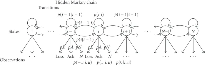
These dynamics are illustrated inFigure 6.
Observations States
· · · Loss Ack N pL pA pN
Loss Ack N pL pA pN p(i|i−1)
p(i−1|i)
p(i−1|i−1) p(i|i) p(i+ 1|i+ 1)
1 · · · i−1 i i+ 1 · · · N−1 N
· · · · · · · · · Transitions
Hidden Markov chain
p(−1|i,u) p(1|i,u) p(0|i,u)
Figure6: An illustration of the model from the point of view of a single source, based on a simple birth-and-death chain for the evolution of the number of active sources.
get the same. This issue is further discussed below, both an-alytically (inSection 3) and in terms of numerical results (in Figure 10).
Another important thing to note is that there are strong similarities between our model and the formalization of mul-tiaccess communication that led to the development of the Aloha protocol. However, the fact that feedback is not broad-cast to all active sources in our model is a major diff er-ence between our formulation and that one. In fact, we con-ceived our model as an analytically tractable “hybrid” be-tween Aloha and TCP. Like in slotted Aloha, time is discrete, feedback is instantaneous, and the state follows a Markovian evolution; but like in TCP, feedback is private only to the source that generated a transmitted packet.
Hajek [24] reviews a series of results for the two usual models for Aloha (finite number of users and one packet at a time, and infinite number of users). Decentralized poli-cies for the injection probabilities, that maintain stability in the case of private acknowledgment feedback, are hard to be derived for the infinite-nodes case with Poisson arrivals. There is however important work [24] about stability in the finite-nodes study of Aloha. The theory in [24] is applied, as an example, to finding conditions of stability for multi-plicative policies for sources that are supplied with Poisson arrivals. We expect that the theory we develop in this paper will provide a useful background for an Aloha model with random arrivals (not necessarily Poisson), with a finite num-ber of backlogged packets, and its extension to the infinite-user model.
2.2. Formal problem statement
Intuitively, what we would like to do is maximizing the rate at which information flows across this queue, subject to the constraint of not losing too many packets. Since each time we attempt to put a packet into the shared buffer there is a chance that this packet may be lost, it seems intuitively clear that without accepting the possibility of losing a few packets, the throughput that can be achieved will be low; at the same time, we do not want a high packet loss rate, as this would correspond to a highly unstable mode of operation for our system.
This intuition is formalized as follows. Our goal is to find a policyg=(u1,. . .,uK) that solves
max g lim supK→∞
1 K
K
k=1
prk=1|xk,uk
,
subject toprk= −1|xk,uk
≤T, ∀k,
(1)
whereT ∈(0, 1] is a parameter that specifies the maximum acceptable rate of packet losses.2Note that we use a lim sup
in the definition of our utility function (instead of a regu-lar limit) because we do not know yet that the limit actually exists—although it certainly does, as will be shown later.
2.3. Warming up: finite horizon and observed state
We start with the solution to an “easier” version of our con-trol problem: one in which the state of the chain (i.e., the number of active sources at any time) is known to all the sources. Although this would certainlynot be a reasonable assumption to make (it does trivialize the problem), we find that looking at the solution to the general problem in this specific case is actually quite instructive, and so we start here as a step towards the solution of the case of true interest (hid-den state).
The problem formulated above is a textbook example of a problem of optimal control for controlled Markov chains, and its solution is given by an appropriate set of dy-namic programming equations [25]. Definec(u) = [p(1 |
i,u)· · ·p(1|N,u)], and then
VK(i)=0, (2)
Vk(i)= sup u:p(−1|i,u)≤T
c(u) +PVk+1
= sup
u:p(−1|i,u)≤T
c(u) +C (Cindependent ofu). (3)
Equation (2) is set to 0 because this is only a finite-horizon approximation, but we are interested in the infinite-horizon
Control
Figure7: Illustrates the separation of estimation and control. Sup-pose we have a controlled system, which produces certain observ-able quantities related to its unobserved state. Based on these obser-vations, we compute aninformation state, a quantity that somehow must capture all we can infer about the state of the system given all the information we have seen so far (this concept will be made rigorous later). This information state is fed into a control law that uses it to make a decision of what control action to choose, and this action is fed back into the system.
case, and in this case, the boundary condition given byVK= 0 has a vanishing effect as we letK → ∞. What is more in-teresting is that from (3), it follows that agreedycontroller is optimal: this is not at all unexpected, since in our model the transition probabilitiesPare not affected by control, only ob-servations are. The interplay among control and the different probabilities of observations are illustrated inFigure 5.
2.4. One step closer to reality: partial information
Definition 1. Denote the simplex ofN-dimensional proba-bility vectors byΠ= {(p1,. . .,pN)∈RN:pi≥0,
N i=1pi= 1}.
The case of partial information (i.e., when the underlying Markov chain cannot be observed directly) poses new chal-lenges. The problem in this case is that Markovian control policies based on state estimates are not necessarily optimal. Instead, optimal policies satisfy a “separation” property, il-lustrated inFigure 7and extensively discussed in [25, pages 84–87].
Formally, an information state πk is a function of
the entire history of observations and controls r0· · ·
rk−1u0· · ·uk−1, with the extra requirement thatπk+1can be
computed from πk,rk,uk.3 A typical choice is to letπk be
p(xk|rk−1,uk−1), the conditional probability ofxkgiven all the past observations and applied controls. Then, an optimal controller for partially observed Markov chains also satisfies a set of dynamic programming equations, but instead of be-ing over the states of the chain (a finite number), these equa-tions are defined over information states [25] (i.e., over all points in the simplex ofΠprobabilities overNpoints):
VK(π)=0,
whereF denotes the recursive updates ofπ, and where the notation Eπ denotes expectation relative to the measureπ.
3Note that this is a very reasonable requirement to make of something that we would like to think of as capturing some notion of state for our system.
A straightforward derivation gives the information-state transition functionF:
withCπka normalizing constant,Pthe transition-probability matrix of the underlying chain, and D(u,r) = diag[p(r | 1,u)· · ·p(r | N,u)] a diagonal matrix. This is essentially the same set of DP equations as before, but where depen-dence on states is removed by averaging with respect to the current information stateπk. And as before, the optimal con-troller is chosen by recording for eachπthe value ofuthat achieves the supremum in the left-hand side of (4). The op-timal control will thus be a function of only the information state,u=g(π).
2.5. Infinite horizon
In the previous sections, we derived the solution for the op-timal control in the case of partial observations when the time horizon is finite. We can get back now to the
infinite-horizon problem stated in (1). The dynamic programming
algorithm becomes a fixed-point system of equations with the unknowns spanning the simplexΠ. Indeed, we start from the finite horizon case:
Assume that the following limits exist for allπ ∈Πand someJ∗:
The DP equation in (9) holds actually under more
general conditions easy to verify for our model [25]. The
transition-probability matrix P does not depend in our
One might attempt to solve the fixed-point system in (9) with an iteration algorithm on a discretized version of the equations system. However, there are practical difficulties to implement and simulate the optimal controller in the partial information case as defined above, having to do with the fact that our state space is the whole simplex of probability dis-tributionsΠ. Our approach to find an approximate solution for the optimization problem (1) is to solve the dynamic pro-gramming system for the finite-horizon case (finiteK), and study the properties of the obtained control policy by numer-ical simulations.
2.6. Numerical simulations
To help develop some intuition for what kind of properties result from the optimal control laws developed in previous sections, in this section we present results obtained in nu-merical simulations. Our approximation consists in choos-ing the maximum control at timekthat still obeys the loss constraint, since this will also maximize the throughput. In Figure 8, we present a typical evolution over time of the in-formation state, inFigure 9, we illustrate how different values of the threshold T influence the behavior of the controller, and inFigure 10, we address the fairness issue raised at the end ofSection 2.1.
In all our simulations, we compare our controller with partial observation, with the optimal genie-aided controller that would be used if the number of active sources were known. Note that the difference between the optimal genie-aided controller and the controller derived by our algorithm is dependent on the two defining parameters of the system: the loss threshold T, and the transition-probability matrix P. Namely, our controller adapts faster to the network con-ditions if the transition matrix P corresponds to a slowly changing Markov chain; on the other hand, the larger the thresholdT implies better adaptation, at the expense of an increased level of losses.
3. PERFORMANCE ANALYSIS
3.1. Overview
3.1.1. Problem formulation
InSection 2, we gave a model for the system of interest, we described its dynamics, we formulated an optimal control problem, we showed how this problem can be solved using standard techniques developed in the context of controlled
Markov chains [25], and we developed numerical
simula-tions to illustrate with concrete examples properties of the queues operating under feedback control. Now, once we have that optimal control algorithm, each source gets to operate the queue based on its local controller, thus resulting in a “decoupling” of the problem, as illustrated inFigure 11.
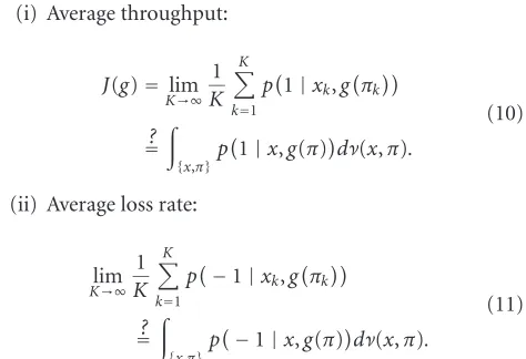
Perhaps the first question that comes to mind once we formulate the picture shown in Figure 11is about ergodic properties of the resulting controlled queues. Specifically, we will be interested in two quantities.
(i) Average throughput:
Therefore we see that, in both cases, the questions of in-terest are formulated in terms of a suitable invariant measure. Since we have assumed the underlying finite-state Markov chain to be irreducible and aperiodic, this chain does admit a stationary distribution. Therefore, a sufficient condition for the existence of the sought measureνis the weak convergence of the sequence of information statesπkto some limit distri-bution over the simplexΠN of probability distributions on
Npoints. And to start developing some intuition on what to expect in terms of the sought convergence result, it is quite instructive to look at typical trajectories of the information state, as shown inFigure 12.
We state now the main theorem of this paper.
Theorem 1. The sequenceπkconverges weakly to a limit dis-tributionνover the simplexΠ.
The proof will follow after we briefly review some previ-ous related work.
3.1.2. Some related work
Note that the stability of the control policy cannot in gen-eral be proven using a Lyapunov function, since the depen-dence of the optimal control on the information state is not a closed-form function.
In view of the previous results [21,22,23], a seemingly feasible approach to establish the sought convergence for our system would have been considering the control action u ∈ U to play the role of a channel input in the setup of [22], while the observations r ∈ O could have played the role of a channel output (thus making the controluand the observationr the available partial observations). However, this approach does not yield the sought result. In our sys-tem, the controluis a function of the information state, that is, it depends on the state of the system, but in those pre-vious papers, inputs are independent of the state of the sys-tem.
3.1.3. Weak convergence of the information state—steps of the proof
The proof of weak convergence ofπinvolves five steps.
1 2 3 4 5 6 7 8 9 10 Number of sources
0 0.2 0.4
Momentk=4; obs.=0
Stat
e
p
ro
babilit
y
1 2 3 4 5 6 7 8 9 10
Number of sources 0
0.2 0.4
Momentk=5; obs.=0
Stat
e
p
ro
babilit
y
1 2 3 4 5 6 7 8 9 10
Number of sources 0
0.2 0.4
Momentk=6; obs.=1
Stat
e
p
ro
babilit
y
1 2 3 4 5 6 7 8 9 10
Number of sources 0
0.2 0.4
Momentk=18; obs.=0
Stat
e
p
ro
babilit
y
1 2 3 4 5 6 7 8 9 10
Number of sources 0
0.2 0.4
Momentk=19; obs.= −1
Stat
e
p
ro
babilit
y
1 2 3 4 5 6 7 8 9 10
Number of sources 0
0.2 0.4
Momentk=20; obs.=0
Stat
e
p
ro
babilit
y
Figure8: Illustrates typical dynamics ofπ. This plot corresponds to a symmetric birth-and-death chain as shown inFigure 6, with probabil-ity of switching to a different statep=0.001,N=10 sources, and loss thresholdT=0.04. At time 0, the initialπ0is taken to beπs(i)=1/N, the stationary distribution of the underlying birth-and-death chain. While there are no communication attempts (up until timek =6),
πkremains atπs. Then at time 6, a packet is injected into the network and it is accepted, and as a result, there is a shift in the probability mass towards the region in which there is a small number of active sources. Then at time 19, another communication attempt takes place but this time the packet is rejected, and as a result, now the probability mass shifts to the region of a large number of active sources. This type of oscillations we have observed repeatedly, and gives a very pleasing intuitive interpretation of what the optimal controller does: keep pushing the probability mass to the left (because that is the region where more frequent communication attempts occur, and therefore leads to maximization of throughput), but dealing with the fact that losses push the mass back to the right. Similar oscillations are also typical of linear-increase multiplicative-decrease flow control algorithms such as the one used in TCP.
πk has the Markov property itself. This is a Markov chain taking values in an uncountable space, though (the simplexΠ).
(2) Then we discretize the simplexΠ. And we show that
for all “small enough” discretizations, there is at least one observation takingπkout of any cell with positive
probability. With this, we make sure that there are no absorbing cells, in the sense that once the chain hits that cell, it gets stuck there forever.
0 100 200 300 400 500 600 Time
0 0.1 0.2 0.3 0.4 0.5 0.6 0.7 0.8 0.9 1
Con
tr
o
l
Desired source Oracle
(a)
0 100 200 300 400 500 600
Time 0
0.1 0.2 0.3 0.4 0.5 0.6 0.7 0.8 0.9 1
Con
tr
o
l
Desired source Oracle
(b)
0 100 200 300 400 500 600
Time 0
0.1 0.2 0.3 0.4 0.5 0.6 0.7 0.8 0.9 1
Con
tr
o
l
Desired source Oracle
(c)
Figure9: Illustrates how the value of the loss thresholdTaffects the optimal control law. In this case, we consider the same birth-and-death model considered inFigure 8, with three different values forT: top-left,T =0.1; top-right,T=0.02; bottom,T =0.05. In all plots, the horizontal axis is time, the vertical axis is control intensity, and two controllers are shown: the thick black line corresponds to our optimal control law, the thin dotted line corresponds to a genie-aided controller that can observe the hidden state. And we observe a number of interesting things: (i) whenTis large (a), our optimal control stays most of the time above the fair share point determined by the actions of the genie-aided controller; (ii) also whenTis large, we see that sudden increases in bandwidth are quickly discovered by our optimal law; (iii) whenTis small (b), the gap between the control actions of our optimal law and the genie-aided law is smaller, but our law has a hard time tracking a sudden increase in available bandwidth; (iv) for intermediate values ofT(c), both the size of the gap and the speed with which changes in available bandwidth can be tracked are in between the previous two cases. These plots also suggest another intuitively very pleasing interpretation:Tis a measure of how “aggressive” our optimal control law is.
we make sure that there is at least one cell which can be reached from any initial point inΠ, and hence that the set of recurrent cells is not empty.
(4) Consider next any “small enough” discretization of the
0 100 200 300 400 500 600 Time
0.3 0.4 0.5 0.6 0.7 0.8 0.9 1
Con
tr
o
l
Maximum Minimum Oracle
(a)
0 100 200 300 400 500 600
Time 0.3
0.4 0.5 0.6 0.7 0.8 0.9 1
Con
tr
o
l
Oracle Desired source
(b)
Figure10: Illustrates the fairness issue raised at the end ofSection 2.1. In this case, we also consider a birth-and-death chain model as in previous examples, but now with only two sources (N =2). In (a), we show the maximum and the minimum control values chosen by either one of the sources over time: thick black line shows the minimum, thin solid line shows the maximum (for reference, the genie-aided controller is also shown); in (b), the thick line corresponds to the control actions of only one of the sources, all the time. Observe how, around time steps 150–250, the source shown at the bottom is the one that achieves themaximumat the top; but around time steps 500–600, the same source achieves theminimumof those injection rates. This is yet another intuitively very pleasing pattern that we have observed repeatedly in many simulations: the control law is essentially fair in the sense that, although we do not have enough information to make sure that at any time instant all controllers will use the same injection rate, at least over time the different controllers “take turns” to go above and below each other.
B(uN) N . . .
B(u2) 2
B(u1) 1
c
Turned into
B(g(π)) N
. . .
B(g(π)) 2
B(g(π)) 1
c(π)
c(π)
c(π)
Figure11: Illustrates how the original problem is broken intoNindependent identical subproblems. Since all the nodes execute exactly the same control algorithm, the distribution ofπis the same for all nodes. But other than through this statistical constraint, all decisions are taken locally by each node, based on private data that is not available to any other node, and therefore completely independent.
of the cells, and therefore it admits an invariant mea-sure itself.
(5) Finally, we construct a measure as the limit of the “simple” measures from step 4 (as we let the size of the discretization vanish), and we show that this limit is invariant overΠ. This requires some further steps, largely based on the elegant framework of [26] as fol-lows.
(5.1) We show that the limit exists and is well defined (it is independent of the particular sequence of dis-cretizations considered).
(5.2) We construct a simpleϕ-irreducibility measure on Π, and from there, we conclude the existence of a
uniquemaximalψ-irreducibility measure. (5.3) We construct a family of accessible atoms inΠ, and
show thatπk is positive recurrent. From this and from 5.2, using a theorem from [26], we conclude that there exists a unique invariant measure onΠ. (5.4) We show that the limit measure of (5.1) is indeed invariant, and therefore conclude that it must be the unique measure of (5.3).
0
Figure 12: Looking at the evolution in time of the information state. For a system with three sources,πis a point in the 2D sim-plex as shown in this figure. And after letting the system run for some time, we find that there are regions of space visited fairly often (bottom right), regions visited less often (bottom left), and regions never visited (top right). Yet each point on this simplex determines a choice of an injection rate, and therefore the frequency with which each point is visited is clearly a fundamental performance analysis tool.
to resort to a more general theory of Markov processes. Meyn and Tweedie provide an excellent coverage of the problem of Markov chains on general spaces [26], which we found to be an invaluable tool in our work.
We continue now with the formal proofs for the steps of the proof above.
3.2. Weak convergence—steps 1–4
Step 1:πis Markov
Although involving a chain defined over a metric space, this proof is elementary, since all we need to invoke is the stan-dard definition of the Markov property and the total proba-bility law: cause when conditioned onπk, we can add in the condition-inguk, sinceuk = g(πk), and the total probability law, and (c) because conditioned on anything else,rk depends only onxk,uk, andπkcontains all information aboutxkgiven the
past. So we see that when conditioning on the past values, πk+1depends only onπk, and henceπis Markov.
An interesting observation to make here—which gives some insight into structural properties of our model that will allow us to prove the sought weak convergence result—is that the intensity of the arrivals process is amemorylessfunction ofπ. Although we have not attempted to prove this, it seems at least intuitively clear to us that if instead of the optimal controller we used a suboptimal one (typically based on the formation of an estimate of the current state), then the op-timal decision would not be a memoryless function of the state estimate, but would actually require past state estimates as well.
Step 2: nonabsorbing small discretization cells
The next step is to show that there is a constantC >0 such that, for any information state π ∈ Π, there exists an ob-servationr ∈Ofor which the distance betweenπkand the next-step information stateπk+1corresponding toris larger
thanC. This allows us toquantizethe simplexΠand make sure that, provided that the size of a quantization cell is small enough, at least one observation will take the current infor-mation state to a different cell.
Lemma 2. There exists a constantCsuch that for anyπ∈Π, there is an observationrfor which π−F[π,g(π),r] ≥, for all0<≤C, and for any norm · .
Proof. This basically means that for any state, there is at least one observation that moves the chain at a finite nonzero dis-tance away from that given state. We prove this by contradic-tion. We show that if all jumps are infinitesimally small, then the only information state that can satisfy this condition is the stationary distribution πs of the original chain. But for this particular information state, any observation different fromr=0 does allow jumps of finite size away from it.
Suppose that for anyC > 0, there exists a pointπ ∈ Π such that for any observationr∈O, π−F[π,g(π),r] < C. Denote byQCthe set of pointsπverifying the above condi-tion for a givenC. Then, ifC1> C2, thenQC2⊆QC1. Denote
by Q0 the intersection of allQC sets. Then the supposition that we want to contradict is equivalent toQ0= ∅.
Consider now anyπ ∈ Q0. Then for any C arbitrarily
close to 0, and for any observationr, π−F[π,g(π),r] < C (all jumps are arbitrarily close to zero).
In what follows,k(·)are normalizing constants. Ifr =0,
it results thatπ is arbitrarily close to πP. This means that πis arbitrarily close toπs(the stationary distribution ofP). Also, forr= −1, orr=1, consider the respectiveD(g(π),r) diagonal matrices. It results that π is arbitrarily close to 1/kπ,rπD(g(π),r)P. Butπis arbitrarily close toπsas well, so it results thatπsis arbitrarily close to 1/k
πs,rπsD(g(πs),r)P. In the limit, πs = 1/k
πs,rπsD(g(πs),r)P. But this cannot be true because D is not the identity matrix. Actually, D is a diagonal matrix with increasing or decreasing diago-nal elements (d1,. . .,dN), forr = 1, respectively,r = −1. If, for example, r = 1, then πs = 1/k
Thespace (0, 0,. . ., 0, 1) −1
π0 1 0
π1 1
−1 0
πk−1 −1
πk 1 0
−1 1 0
πk+1
πs
ε−cell
(1, 0, 0,. . ., 0)
Figure13: A sequence ofr=0 observations leads the chain arbi-trarily close toπs.
This would mean that there existsπ1 =1/kπs,1πsD(g(πs), 1) withπs=π
1P. We know thatπs=πsP, so if the chain
ad-mits only one stationary distribution, it results thatπ1=πs.
However this is not possible, since πsD(g(πs), 1) moves to-wards (1, 0,. . ., 0) the mass function of the new probability vector with respect toπs.
Step 3:πsis reachable from anywhere
Lemma 3. For anyπ∈Π, there is a nonzero probability that in the limit, the chain reaches arbitrarily close to the stateπs, when starting in stateπ.
Proof. We illustrate inFigure 13the intuition on which we base our proof. The proof relies on the observation that finite-length sequences ofr =0 observations move the state arbitrarily closer toπs. If the observation at timekisr
k=0,
then the matrix D(uk,rk) becomes diagonal with elements
dii=1−uk, so it equals the identity matrix multiplied with a constant; then the recursion for the information state, when-ever the source decides not to transmit, can be expressed as πk+1=πkP. This vector equation has as solution the station-ary distributionπs. It follows that for anyπ ∈ Πas initial state of the chain, there is a path by which the chain reaches in the limit the stationary distribution stateπs, via for example a sequence of successiverk=0 observations. But any arbitrary finite-length sequence ofrk = 0 observations may happen with nonzero probability, so for anys >0, there is a finite timeKwithrk=0,k≤K, in which the chain can reach with nonzero probability a stateπssuch that πs−πs ≤s.
Step 4: positive recurrent discretization on a nonempty subset
We consider now quantizations of the Markov chain formed by the sequence of information states, with quantization cells of size ≤ C. If the cell size is small enough, then from Lemma 2, it follows that for any π inside a discretization cell, there is at least one observation happening with nonzero probability for which the chain jumps outside the cell. This ensures that there is no state of the chain in which the system stays forever, so the recurrent irreducible subset of discretized cells has more than one element. With this procedure, we define a family of quantizations ofΠ, with members of the family of the form q = {q1,. . .,qN}, whereq
i are theN compact sets contained in q andiqi = Π,
iqi = ∅. For simplicity, we will denote byq(π) the cell to which the instantaneous information stateπbelongs. We note that
pqk+1|qk,qk−1,. . .
=
πk+1∈qk+1,πk∈qk,πk−1∈qk−1,...
pπk+1|πk,πk−1,. . .)dπk+1dπkdπk−1. . .
=
πk+1∈qk+1,πk∈qk
pπk+1|πk
dπk+1dπk
=pqk+1|qk
(13)
since the process πk is Markov. The measure with respect to which we are integrating is Lebesgue measure over theΠ space. We just count how often the continuous chain falls in a given cell. Thus the processq(πk) forms afinite-statechain, also having the Markov property (inherited from the contin-uous chain).
Lemma 4. For any ≤ C, there is a subsetP ⊆ Π, which
contains the stationary distributionπsof thex
koriginal chain, and on which the discretized chainq(πk)is positive recurrent.
Proof. We show inFigure 14a typical behavior of the chain,
that shows the existence of a recursive subset P ⊆ Π. We base our proof on the fact thatπsis recurrent so its proper-ties will be induced on a recurrent closure of the discretized version of the simplexΠ. As we showed inLemma 3, the in-formation stateπscan be reached in the limit with nonzero probability from any π0 initial state of the Markov chain.
For any initialπ0, there is a sequenceπ0,. . .,πk,. . . such that
Thespace (0, 0,. . ., 0, 1)
Figure14: After passing through a sequence of transient states, the chain reaches a recursive subset of the discretized simplexΠ.
Denote byPthe set of reachable quantization cellsq(π) if the chain starts inπs. We already proved that the cell con-tainingπsis accessible in a finite number of steps from any other information stateπ, so implicitly from any cellqi ∈P as well. Moreover, by construction, any cellqi ∈Pis reach-able fromq(πs). Since ≤C, then for anyq(π
k), there is at least one observationr for which the transition from πk toπk+1 leads toq(πk+1)=q(πk). It follows that the chain with states inP is irreducible (and aperiodic as well, since the cell containingπsis one-step reachable from itself, via an
r = 0 observation). The state space is finite, so the chain is positive recurrent, and thus it has a stationary distribution. Denote by pthis probability distribution over thePstate space. Ifqi ∈/ P, thenp(qi)=0.
We will prove now that there is a limit probability mea-sure onΠto whichpconverges in the limit→0, and study the properties of that measure.
3.3. Weak convergence—step 5
There exists a unique limit invariant measure overΠ,ν→ν,
when→0.
Step 5.1: existence of the limit measure
We will show that the limit measure exists by considering, for any subsetAofΠ, sequences of measures on subsets of the discretized simplex that cover, and respectively, intersectA. We show that they converge to the same limit.
Definition2. Define theinnerandoutersequences of
mea-sures over the simplex Π, corresponding to the set of
-discretizations: our limit invariant measureν(A).
We will prove first convergence of each of the limits. Con-siderνI
; we will prove that the sequence is Cauchy for any set
A, and it trivially has a convergent subsequence, which will mean that the whole sequence is convergent.
For a given set A, denote byAn = {∪S ∈ Pn : S ⊆ A}the inner cover of setAcorresponding to discretization stepn. We will prove first that the normalized volume of the difference set between two inner covers of the setAtends to the empty set, and consequently the probability measure over that difference set tends to zero. Define the metricd(X,Y)=
µLeb((X−Y)∪(Y−X))/µLeb(Π), on theσ-algebraBofΠ,
X,Y ∈B(this represents the normalized volume of the set where the two subsetsX,Y differ from each other—µLeb is
Lebesgue measure). It is easy to verify thatd(·,·) is indeed a valid metric.
Letn be a decreasing sequence of discretization steps, with limn→∞n = 0. Then due to the fact thatPn is a
se-quence of subsequent discretizations of the space Π when
n → ∞, it follows that limn→∞An = A. SinceAnis conver-gent, it is also Cauchy in the metric space (B,d). This means that for anyδ > 0, there existsnδsuch thatd(An,Am)< δ, for anym > n≥nδ. So the normalized volume of the set dif-ference between two set elements of the sequence becomes arbitrarily small. That also means that ifn,m → 0, then
νI
nm(d(An,Am)) → 0, as νnm is a stationary distribution over finite spaces with decreasing cell size. Then for anyδν> 0, there isnδνsuch thatνInm((An−Am)∪(Am−An))< δν, for measures (sum of probabilities of-discretization cells that cover exactly an-discretization cell is equal to the proba-bility of that -discretization cell), and the wayAn,Am are constructed (cells corresponding to multiples ofare all in-cluded in the cells corresponding to).
We conclude that for anyδν > 0, there isnδν such that
|νI
n(An)−ν I
m(Am)|< δν, for anym > n ≥nδν. This means that the sequence νI
n(An) is Cauchy as well. It is trivial to show that there is a convergent subsequence ofνI
n(An). Pick, for example, n = 0/2n, then the corresponding
subse-quence is bounded from above by 1, and monotonically in-creasing; it follows that the subsequence is convergent. But a Cauchy sequence with a convergent subsequence is conver-gent, which proves thatνI
(A) is convergent for any setA. The proof for convergence ofνO
is similar and we will omit it. Both limits exist, and it is obvious that they fulfill the inequality
lim →0ν
I
(A)≤lim→0νO(A), for anyA⊂Π. (15)
We want to prove that the inequality above holds in fact with equality. Assume that the inequality is strict; then let δ=νO
0(A)−νI0(A)>0. But this would mean that there exists
Definition3. Define the measureνover the simplexΠas the common limit of the two sequences of measures:
ν(A)=lim →0ν
I
(A)=lim→0νO(A) (16) for a givenA⊆Π.
For the proofs in the next two sections, we will use defi-nitions and notations also found in [26].
Step 5.2: existence of a unique maximal ψ-irreducibility measure
Definition4. Denote byB(π0,δ)= {π∈Π: π−π0 < δ}
the open ball, withδ >0.
Definition 5. Denote byB(Π) theσ-field generated by the open balls inΠ.
Definition 6. Denote, for any stateπ ∈ Πand subsetA ∈ B(Π), the probability that, when starting in stateπ, the chain reaches subsetA:
L(π,A)=Pπ
τA<∞
. (17)
Lemma 5. Letπn∈Π,n=0, 1,. . .be a sequence of informa-tion states. Thenπnisφ-irreducible onB(Π).
Proof. Letπsbe the stationary distribution of the underlying chain. Define the measureφonB(Π) as
φBπs,δ=µLebBπs,δ,
φ(A)=0 otherwise. (18)
In step 3 of the proof, we proved thatπsis reachable from anywhere. Hence, for allπ∈Π, we haveL(π,B(πs,δ))>0, andφis an irreducibility measure.
Note. If aφ-irreducibility measure exists, then there is a part of the space reachable from anywhere, so one might expect independence of the chain from the initial conditions, by analogy with finite chains.
Proposition 1. Ifπnisφ-irreducible, then there exists a unique “maximal” measureψonB(Π)such thatπnisψ-irreducible andφ≤ψ. Denote byB+(Π)theσ-algebra ofΠwith sets on
whichψis positive.
Proof. The proof involves concepts outside the scope of this paper, but is standard for chains fulfilling the previous con-ditions, and it can be found in [26].
Step 5.3: uniqueness of the invariant measure onΠ
Definition7. α∈B(Π) is called anatomfor a sequenceπnif there exists a measureµonB(Π), such that, for anyπ ∈α, P(π,A)=µ(A) (for anyA∈B(Π)).
Definition8. αis called anaccessible atomfor a sequenceπn, ifπnisψ-irreducible andψ(α)>0.
Note. Atoms behave like states in finite chains. From the de-velopment in [26], it turns out that the reason why so many results about finite chains carry over to more general set-tings is precisely the fact that it is always possible to construct atoms.
Proposition 2. All balls B(πs,δ), with δ > 0, are accessible atoms for any sequenceπn.
Proof. Letαbe a set inB(Π), and letπ∈α. Then, depending on the current observationr, there are three possible transi-tions fromπ, via the recursion functionF[π,g(π),r]. Then for anyA∈Π, we can consider the measure
µ(A)=p(r) ifFπ,g(π),r∈A,
µ(A)=0 otherwise. (19)
Then anyα=B(πs,δ) is an accessible atom.
Definition9. Denote byEπ[ηA] the expected number of re-turns of the chain to subsetA∈Πwhen starting in stateπ.
Definition10. A setA∈B(Π) is calledrecurrentifEπ[ηA]= ∞for allπ∈A(when starting inA, the expected number of returns toAis infinite).
Lemma 6. Ifπnisψ-irreducible and admits a recurrent atom
α, then every set inB+(Π)is recurrent.
Proof. IfA∈B+(Π), then for anyπ, there existr,ssuch that
Pr(π,α)>0,Ps(α,A)>0 and we can write, by considering the paths of the chain that go fromπtoAvia the atomα,
n
Pr+s+n(π,A)≥Pr(π,α)
n
Pn(α,α)
Ps(α,A)= ∞.
(20)
Since α, being an atom, implies that nPn(α,α) diver-ges.
Note. Observe again the analogy between atoms and states of a finite chain.
Definition 11. A sequenceπnis calledrecurrent if and only if it is ψ-irreducible, andEπ[ηA] = ∞for anyπ ∈ Πand
A∈B+(Π).
Lemma 7. Any sequence of information states drawn from the Markov chainπnis recurrent.
Proof. FromLemma 5and Proposition 1, it results thatπn is ψ-irreducible. Furthermore, from step 3 of the proof, it results that all the balls B(πs,δ), with δ > 0, are recur-rent atoms. Then everyA ∈ B+(Π) is recurrent, and from
Definition 10, it results that Eπ[ηA] = ∞ for all π ∈ A. We still need to prove that even if π /∈ A, we still have L(π,A) = 1. By definition, L(π,B+(Π)) = 1. Suppose
IfA=B, then the sought result follows. Otherwise, we will haveL(y,A)>0 for ally∈B, because of theψ-irreducibility overB+. ButB∈B+(Π) andE
y[ηB]= ∞, so it results that
L(y,A)=1. So finally,L(π,A)=1 and this case is reduced to the previous one (whereπ∈A). Hence,πnis recurrent.
Definition12. A sequenceπnis calledpositiveif and only if it isψ-irreducible and admits an invariant measureγ.
Lemma 8 (Kac’s theorem). If a sequenceπnis recurrent and admits an atomα∈B+(Π), thenπ
nis positive if and only if
Eα[τα]<∞.
Proof. IfEα[τα]<∞, then obviouslyL(α,α)=1, so it results
πn is recurrent. It also results from the structure ofγ (see [26]) thatγis finite, so is positive as well. The converse results from the structure ofγas well.
Lemma 9. The sequence of information statesπnis positive.
Proof. From Lemma 7, it results that πn is recurrent. Also, from step 3 of the proof, it results that every ball α =B(πs) ∈ B+(Π) is an atom, andE
α(τα) < ∞. Then it results thatπnis positive.
Theorem 10. There exists a unique invariant probability mea-sure ofπn.
Proof. The proof for this theorem is valid for chains having the properties we have analyzed until now, and can be found in [26].
Step 5.4: invariance ofν
We prove nowTheorem 1. The measureν(as constructed in step (5.1)) is the unique invariant probability measure onΠ.
Proof. For invariance ofν, we need to prove that
ν(A)=
Πν(d y)P(y,A). (21)
From the definition ofν, we have that for any>0,
νI
(A)≤ν(A)≤νO. (22)
If we denote byP(·,·) the transition-probability kernel for the-discretization, then we can rewrite the rightmost term of the inequality (22) as
νI (A)=
S∈P:S⊆A p(S)
=
S∈P:S⊆A
T∈P
p(T)P(T,S)
=
T∈P
S∈P:S⊆A
p(T)P(T,S)
=
T∈P
p(T)PT,∪S∈P:S⊆A.
(23)
In a similar manner, we can rewrite the expression for νO
(A):
νO (A)=
T∈P
p(T)PT,∪S∈P:S∩A= ∅. (24)
By taking now the limit in expression (22), we know that both left and right limits exist and are equal, so it results that
ν(A)=lim →0
T∈P
p(T)PT,∪S∈P:S⊆A
=lim →0
T∈P
p(T)PT,∪S∈P:S∩A= ∅
(a)
=
Πν(d y)P(y,A),
(25)
where equality (a) holds because, under some continuity
conditions, in the limit → 0, the sum becomes integral;
the probability limit νexists; the quantization cell T ∈ P becomes the infinitesimal integration variableT →d y; the transition-probability kernelP(·,·)→P(·,·); and both the reunions of cells included inAand, respectively, intersecting Acover whole setA.
It results thatνis invariant, and thus it is the unique in-variant measure onΠ.
3.4. Numerical simulations
In this section, we show results of numerically evaluating the integrals above. We simulated a system withN =2,N =4, and N = 8 sources, and with different values for the loss threshold T = 0.02, T = 0.05, and T = 0.1. The chain is birth-and-death with probability Pswitch. We let the
sys-tem run for t = 100 000 time steps. We plot the average
throughput and loss as a function of the transition probabil-ityPswitch. The resulting plots are shown inFigure 15. We see
that the plots do not depend significantly onPswitch. The
de-pendence is essentially on the stationary probabilityπsof the original chainP, which is the same for any symmetric birth-and-death chain. As expected, large values forTimply larger throughput, as the controller is allowed to probe more often the environment; this is on the expense of increased losses.
4. CONCLUSIONS
0.05 0.1 0.15 0.2 0.25 0.3 0.35 0.4 0.45 0.5
Figure15: The plots from up to bottom:N =2, 4, 8 sources. Left: average throughput; right: average loss. Legend: dotted plot,T =0.1; dashed plot,T=0.05; solid plot,T=0.01.
tackle these problems was that by conditioning on informa-tion states, the arrivals process does become a process with independent increments—but since this conditioning term is itself Markov, this is how the model is rendered analytically tractable.