Smooth eigenvalue correction

R E S E A R C H

Open Access

Smooth eigenvalue correction

Anne Hendrikse

, Raymond Veldhuis

and Luuk Spreeuwers

Abstract

Second-order statistics play an important role in data modeling. Nowadays, there is a tendency toward measuring more signals with higher resolution (e.g., high-resolution video), causing a rapid increase of dimensionality of the measured samples, while the number of samples remains more or less the same. As a result the eigenvalue estimates are significantly biased as described by the Marˇcenko Pastur equation for the limit of both the number of samples and their dimensionality going to infinity. By introducing a smoothness factor, we show that the Marˇcenko Pastur

equation can be used in practical situations where both the number of samples and their dimensionality remain finite. Based on this result we derive methods, one already known and one new to our knowledge, to estimate the sample eigenvalues when the population eigenvalues are known. However, usually the sample eigenvalues are known and the population eigenvalues are required. We therefore applied one of the these methods in a feedback loop, resulting in an eigenvalue bias correction method.

We compare this eigenvalue correction method with the state-of-the-art methods and show that our method outperforms other methods particularly in real-life situations often encountered in biometrics: underdetermined configurations, high-dimensional configurations, and configurations where the eigenvalues are exponentially distributed.

1 Introduction

In data modeling, in order to give a meaningful interpreta-tion of input samples, a descripinterpreta-tion of the data generating process is needed. Often little is known about this pro-cess beforehand and the description consisting of a model and its parameters has to be derived from a set of exam-ples, called the training set. Since the number of samples is usually limited in this training set, a model is cho-sen beforehand: The generation of this set is modeled as drawing samples from a random processP(x), where the distribution of this random process is approximated by a multivariate normal distributionN(μ,).

There are two reasons for modeling the distribution withN(μ,). Firstly, a normal distribution has the high-est entropy for a given variance. Therefore, according to the principle of maximum entropy, the normal distribu-tion is the best choice if no further informadistribu-tion about the distribution is available [1]. Secondly, for a multivariate normal distribution, only the second-order statistics have to be determined. the estimates of higher-order statistics in high-dimensional data can be highly distorted as shown

*Correspondence: [email protected]

1Signals and Systems Group, EWI Department, University of Twente, Hallenweg 15, 7522NH Enschede, the Netherlands

in [2], but, as we will show, even the estimation of the second-order statistics may be severely distorted.

As mentioned before, the parameters of the distribution N(μ,), thepopulation meanandpopulation covariance matrix, are usually unknown and have to be estimated from the training samples. For the mean, the sample mean,

ˆ

μ= 1 N

N

k=1

xk, (1)

and for the covariance matrix, the sample covariance matrix,

ˆ

= 1 N−1

N

k=1

xk− ˆμ

·xk− ˆμ T

, (2)

are often used as estimates. HereNis the number of sam-ples in the training set, where each sample is a column vector withpelements, denoted byxk.

It is known that thesample distributionN

ˆ

μ,ˆ

is not a good estimate of thepopulation distributionN(μ,) ([3] or see for example our demonstration in [4]), because even though the elements of the sample covariance matrix are unbiased estimates of the elements of the population

covariance matrix, the eigenvalues of the sample covari-ance matrix, thesample eigenvalues L= {lk|k = 1. . .p}, are biased estimates of the eigenvalues of the population covariance matrix which are the population eigenvalues = {λk|k = 1. . .p}. In [5] it has even been suggested to abandon the estimation of ˆ altogether. In classical (LSA), sample eigenvalues seem unbiased because it is assumed that the number of samples is large enough to fully determine the statistics of the sample covariance matrix.

However, many applications evolve in such a way that the dimensionality of the sample space increases as fast as or even faster than the number of samples in train-ing sets. For example, in face recognition, the resolution of face images has increased considerably because high-resolution devices have become available at modest costs, and the dimensionality of the sample space is related to the image resolution. The number of training samples depends on the number of test subjects available and the effort that can be put in collecting the data. As a result, in one of the databases with the largest number of sub-jects, the FRGC2 database [6] has images of approximately 500 individuals, while the feature vectors can easily reach a dimensionality of 10,000.

If the dimensionality is in the same order or even higher than the number of samples, (LSA) no longer gives accu-rate predictions of the statistics of the estimators. In (GSA) the dimensionality of the samples is also consid-ered and is therefore more applicable than (LSA) as will be discussed in Section 2.1.

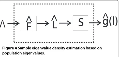
Building on the work of many as is described in [7] using (GSA), a relation between the sample eigenvalues and population eigenvalues was determined for a narrow set of sample distributions in[8], the Marˇcenko Pastur equation. In [9] it was shown that this relation holds for a large set of distributions. Based on this relation in case of largep andN, a correction of the sample eigenvalues is possible which leads to a more accurate estimate of the population eigenvalues. The basic idea is shown in Figure 1.

In Figure 1 the first part models how the sample eigen-values are obtained. In the model, the data-generating process generates samples for a training setXby drawing

samples from a normal distribution with a set eigenval-ues, thepopulation eigenvalues. From the training set a sample covariance matrixˆ is estimated. The decompo-sition of the matrix results insample eigenvaluesL. This process can be modeled as a function B() = L. Bias correction can then be interpreted as applying an esti-mate of the inverse ofBto the sample eigenvalues, which results in ˆc, the estimate of the population eigenvalues after correction.

One aspect of analyzing eigenvalue estimation with (GSA) is that eigenvalue estimation is considered in the limit that the dimensionality of the samples becomes infinitely large. Therefore, instead of considering the eigenvalue set, an eigenvalue distribution description is used as explained in Section 2.1. The Marˇcenko Pastur equation in fact does not give a relation between the sample eigenvalues and the population eigenvalues, but between the corresponding distributions in the (GSA) limit.

Of course, in practice, the dimensionality of the sam-ples and the number of samsam-ples are not infinite, and the Marˇcenko Pastur equation cannot be used directly to cor-rect the bias in the sample eigenvalues. However, as we will show in Section 2.4, by applying a smoothing oper-ation to both the populoper-ation distribution estimate and the sample eigenvalue distribution estimate, the relation between the two smoothed distributions is still accurately described by the Marˇcenko Pastur relation.

Because the Marˇcenko Pastur equation does relate the two smoothed distributions, we could develop two meth-ods in Section 2.5, a polynomial method and a fixed point method, which both give a smoothed estimate of the sam-ple eigenvalue density given a set of population eigenval-ues. But in practice, bias correction is often desired, which equals to estimating the population eigenvalues corre-sponding to a set of sample eigenvalues. In Section 2.6 we derive two methods that can estimate a set of population eigenvalues given a set of sample eigenvalues. The fixed point bias correction method uses the fixed point sample eigenvalue density estimator, which shows that population eigenvalue to sample eigenvalue estimators do have their application.

In Section 3 we present several experiments. First we illustrate the effectiveness of the two sample eigenvalue density estimation methods: We show that the polynomial method makes good estimates of the sample eigenvalue densities if the number of population eigenvalue clusters is low, but fails if that number increases. Second we also show that the number of required iterations of the fixed point method increases if we decrease the smoothness of the estimation.

We then compare the fixed point bias correction method with a state-of-the-art bias correction method by Kaorui [7] and a bootstrap bias correction method we pre-sented in [10]. The fixed point method performs well in all experiments and excels in two real-life examples we often encountered in biometrics. In Section 4 we present conclusions based on these experiments.

2 Bias of the sample eigenvalues

2.1 Large sample analysis of eigenvalue bias

Bias is a statistic of an estimator and in order to find the statistics of estimators, often the classical (LSA) is performed. In (LSA) the statistics of an estimator are determined for the limitN → ∞, whereNis the num-ber of samples. With (LSA), the sample eigenvalues seem to be unbiased. However, in many applicationsNis of the same order as the dimensionality of the sample space,p and (LSA), which provides inaccurate statistics.

2.2 General statistical analysis of eigenvalue bias

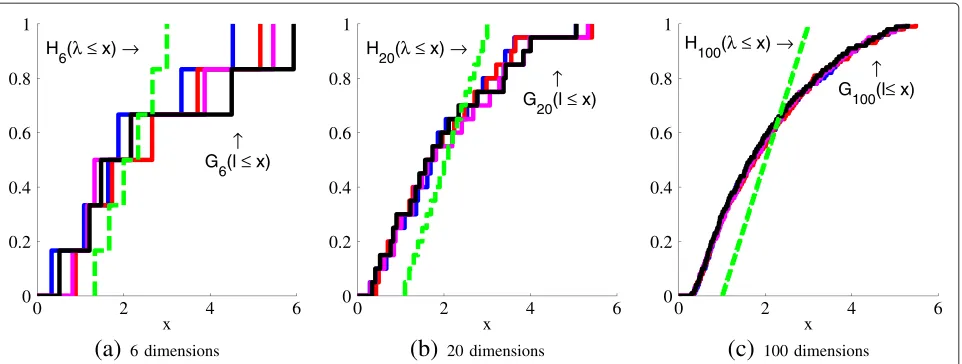
In (GSA) [11] the limitN,p→ ∞while_Np →γ is consid-ered, whereγ is some positive constant. Applying (GSA) to eigenvalue estimation does show a bias in the estimates. In the following example we demonstrate the situation under consideration in (GSA). In the example we mea-sured the sample eigenvalues of synthetic data, with the population eigenvalues uniformly distributed between 1 and 3. To show that the (GSA) limit ‘ifp → ∞’ is rele-vant we setpto 6, 20, and 100, while keepingγ = 1₃, so N = 18, 60, and 300, respectively. From the population eigenvalue sets and the measured sample eigenvalue sets, we determined the empirical eigenvalue distribution func-tion, which is given by Equation 3 for an eigenvalue set

xk|k=1. . .p

:

Fp(x) = 1 p

p

k=1

u(x−xk), (3)

where u(x)is the unit step function.

In Figure 2 we show both the empirical population eigenvalue distribution Hp and four empirical sample eigenvalue distributionsGpfor the different settings ofp. Ifpis low, large variations in theGps occur and the bias is only a small component in the estimation error. However, if p increases, the Gps converge to a fixed distribution,

which is different fromHp. This difference is due to the bias in the eigenvalue estimates.

In [8] an equation was given, which describes the rela-tion between the sample eigenvalue distriburela-tions and the population eigenvalue distribution. Originally this rela-tion, here after referred to as the (MP) equarela-tion, was proved for a very limited set of data distributions, but based on the work of many others as described in [7] and in [9], it was shown that the same relation holds for a much larger set. The (MP) equation requires the Stieltjes transform of the empirical sample eigenvalue distribution, which is given by

mGp(z) =

dGp(l)

l−z , forz∈C

+_{. (4)}

Assuming zero mean data, modeled by a randompbyn matrixxin [7], the (MP) equation is given usingvGp(z), the Stieltjes transform corresponding to the spectrum of x∗x/n.vGp(z) is related tomGp(z), which is the Stieltjes transform ofxx∗/n, via

vGp(z) =

1− p n

₋₁

z + p

nmGp(z). (5) As is discussed in [9] both transforms could be used, as the two spectra only differ in(n−p)zero-valued eigen-values. It is argued that the form withvGp(z) makes the study of analytical properties more simple. Notation wise, this form also results in more compact expressions. Note that with finite sample analysis, which will be discussed in the next section, this choice of representation is not that arbitrary and depends on whethern>p.

We now quote Theorem 1 from [7], which gives the (MP) equation and the conditions under which it holds: Theorem 1. Suppose the data matrix X can be written

X = Y

1 2

p, where p is a p×p positive definite matrix

and Y is an n×p matrix whose entries are independent and identically distributed (real or complex), with EYi.j

=0, EYi,j2

=1and EYi,j4

<∞.

Call Hpthe population spectral distribution, i.e. the

dis-tribution that puts mass 1/p at each of the eigenvalues of the population covariance matrix,p. Assume that Hp

converges weakly to a limit denoted H∞(we write this con-vergence Hp ⇒ H∞). Then, when p,n → ∞and p/n →

γ,γ ∈(0,∞),

1. vGp→v∞(z), A.s., wherev∞(z)is a deterministic function

2. v∞(z)Satisfies the equation

− 1

v∞(z) = z−γ

λdH∞(λ)

1+λv∞(z),∀z∈C +

(6)

0 2 4 6 0

0.2 0.4 0.6 0.8 1

x H

6(λ ≤ x) →

↑

G

6(l ≤ x)

(a)

0 2 4 6

0 0.2 0.4 0.6 0.8 1

x H

20(λ ≤ x) →

↑

G

20(l ≤ x)

(b)

0 2 4 6

0 0.2 0.4 0.6 0.8 1

x H

100(λ ≤ x) →

↑

G

100(l≤ x)

(c)

Figure 2Examples of eigenvalue estimation bias toward the GSA limit.The dashed line indicates the population distributionHp, the four solid

lines are the empirical sample distributions ofGp.

Equation 6, the (MP) equation, fully characterizes the sample eigenvalue distribution G∞ if the population eigenvalue distribution is known. However, the question at hand is to derive a method that reduces the bias in the sample eigenvalues, that is, rewrite Equation 6 in the form =B−1(L).

2.3 Finite sample analysis of eigenvalue distribution

Both (LSA) and (GSA) apply limit analysis to find a rela-tion between the popularela-tion eigenvalue set and the sample eigenvalue sets. However, for several data distributions, results are available for the eigenvalue distribution for the limited N and p case. For classes of random com-plex Gaussian vectors, the distributions of the eigenvalues of the covariance matrices have been found, and these results are applied in for example wireless communica-tion. A review of much of the work on this topic is given in [12]. Based on the work in that field, in [13], the joint (CDF) of the eigenvalues of complex Wishart (for the case n > p) and pseudo-Wishart (n ≤ p) random matrices, where the common covariance matrix are found, can take the form of an arbitrary full-rank Hermitian matrix.

These results rely on the assumption that the data can be modeled as proper complex Gaussian random vec-tors (Section II in [14]), which is not the case if the data have only a real component. Indeed, the results on the distribution of the eigenvalues of Wishart matrices of real data derived in [15] and [16] differ consider-ably, suggesting that in the finiteN case, the bias in the sample eigenvalues depends on whether the data is real or complex.

In comparison to the (GSA) analysis, the finite sample analysis have strong requirements on the distribution of the data. Verifying the distribution of the data seems to

become harder as the dimensionality increases (see for the discussion on Gaussianity in [2]), therefore increasing the risk of using the wrong distribution assumption. On the other hand, the rate of convergence to the results of the (GSA) analysis is still an active research topic (Section 3.2 in [3]), although some results sug-gest some error measures decrease by an order ofN−14_.

Nonetheless, the question of when to switch from the finite sample analysis to the (GSA) limit is still an open question.

In our experiments with the Muirhead eigenvalue cor-rection [16], we found that for a dimensionality in the order of a few 100, the correction already had significant distortions, and strong modifications to the correction method had to be made [17]. We therefore continue to use the (GSA) analysis and derive methods from those results.

2.4 Smooth eigenvalue estimation

The Marˇcenko Pastur equation describes the relation between the sample eigenvalue distribution and the population eigenvalue distribution in the (GSA) limit, but in practice both N and p are finite. However we assume that the global characteristics already converge for lower values of N and p, and higher values of N and p are only required if very local details have to be considered. To support this assumption we con-sider the curves in Figure 2 again. The empirical dis-tribution function is always staircase shaped as shown in 2a, with at most p jumps of at least height 1_p, so that the curve can only contain local details if p is large enough. For an exact definition of local detail, see Appendix 4.

by varying the imaginary value ofz, we can control the influence of local details and global characteristics in Equations 6 and 4. We will use this result later on to derive algorithms which can be used in practical situations.

First we introduce the inverse Stieltjes transform:

g(x) = 1

πlimy↓0

mG(x+ıy)

. (7)

In order to find the sample eigenvalue density given the population eigenvalue distribution, Equation 6 has to be solved with {z} ↓ 0. However, as long as we use empirical distributions, setting {z} =0 will lead to sev-eral problems. For example, the Stieltjes transform of the empirical sample eigenvalue distribution will become infi-nite at the sample eigenvalues and real valued anywhere else. If, on the other hand, we solve Equation 6 with {z} with some fixed positive constanty, we find the empiri-cal sample eigenvalue density convolved with the Cauchy kernel_π1_x2₊y_y2

, as noted in [3].

The factorytherefore seems to have a smoothing effect: local details are filtered out. But this is not limited to the resulting density; setting y as non-zero has a sim-ilar effect on the Marˇcenko Pastur equation. Consider the integrands in both the integral of the Stieltjes trans-form (Equation 4) and the integral in the Marˇcenko Pastur equation (Equation 6). Both arguments can be rewritten to the form

b (r)= 1

r−ıq, (8)

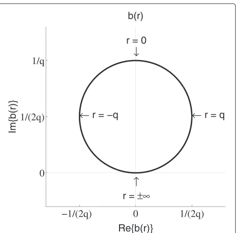
whereris a real variable andqis a real constant. For exam-ple, if we setr = l− {z} andq = {z} we have the argument of the integral in Equation 4. The function in equation 8 is a generalized circle, a specific kind of Möbius transform [18], which in this case describes a circle in the complex plane with a centerı_2q1 and radius _2q1 (see Figure 3).

The result of the integrals in Equations 4 and 6 is deter-mined by the mapping of the distribution function along this circle. In case q is small, only a small part of the real axis is mapped to other positions than the infinity points. If any probability mass is repositioned, it will still be mapped to the infinity points and so the change will have little effect on the result of the integral, unless the change is in the neighborhood aroundr=0. So for small q, the results of the integrals are only sensitive to a small part of the density function.

If on the other hand q is large, much more of the real axis is mapped to other positions than the infinity points. In that case changes of position of density in a large neighborhood aroundr = 0 have an effect on the result of the integral. In the extreme cases, forq ↓0, the integration result is determined by one point on the dis-tribution curve, which gives an explanation of the limit in

−1/(2q) 0 1/(2q)

0 1/(2q) 1/q

↑

r =

← r = −q r = 0

↓

← r = q

Re{b(r)}

Im{b(r)}

b(r)

Figure 3The integration arguments used as mapping functions describe a circle in the complex plain with diameter1_q.Where each pointpis mapped depends on the value ofq: ifqis small, most points will be mapped in the neighborhood ofr_{= ±∞}, if q is large more points will be mapped away fromr= ±∞.

the inverse Stieltjes transform. Ifq → ∞, the results are solely determined by the means of the distributions. An exact proof of these claims is given in Appendix 1.

Because of this mapping the result of the integral is bounded by the circle (see the proof in Appendix 2), which is a more strict property than the well-known condition

{mG(z)} ≤1/{z}[19]. This limit is used for choosing a starting point in the fixed point algorithm in Section 2.5.2, and the limit is also used as an upper bound of the min-imal value of (z) for which the fixed point algorithm converges Appendix 3).

The observation about the sensitivity of the integral results for variations of the distributions is used in the fol-lowing sections where we first derive an algorithm to find a smoothed estimate of the sample eigenvalues if the pop-ulation eigenvalues are known. We then use this algorithm in a feedback algorithm to find an estimate of the pop-ulation eigenvalues given that the sample eigenvalues are known.

2.5 From population eigenvalues to sample eigenvalues

If we substitute the empirical population distribution function Hp(λ) = 1_pp_k=1u(λ−λm) and vˆp(z) for the population distribution and v_∞(z) respectively in Equation 6, we get the following equation:

−1

ˆ

vp (z) =

z− 1 N

p

k=1

λ_k 1+λkˆvp (z)

. (9)

To find the corresponding sample eigenvalue density

ˆ

g(l),vˆp(z)has to be solved from Equation 9. We present two solutions: a polynomial method and a fixed point method.

2.5.1 Polynomial method

In this section we will derive and analyze a polynomial method, which was already found by Rao and Edelman [20]. Their derivation has a solid embedding in random matrix theory, but it is less focussed on the application we discuss in this article.

We derive the polynomial method by rewriting Equation 9 to a polynomial expression by multiplying both sides of the equation withˆvp(z)p_k=1

1+λ_kvˆp(z)

. The new expression can be rewritten to an expression of the form 0 = p_k=+₀1ckvˆkp(z), which then can be solved using standard polynomial solving tools.

A problem with this method is that if the number of eigenvalues increases, the order of the polynomial increases and the roots of the higher order polynomial become numerically unstable. As observed in the experi-ments, the polynomial solution becomes unreliable above 10 eigenvalues. The advantage of the method is that it can solve Equation 9 for arbitrarily small {z}values, even 0.

The numerical issues with root finding is a well-known problem. Wilkinson, for example, demonstrated it in [21]. One approach to mitigate the numerical dependency on the coefficients of the polynoom is to use a basis dif-ferent from the monomial basis. This has been demon-strated successfully in polynomial approximation by using Lagrange polynomials in [22]. As the outcomes are lim-ited by a circle as described in Section 2.4, maybe a similar approach as used in the Lindsey-Fox method [23] could be used. However, this large field of study is beyond the scope of this paper, so we do not go further into this subject.

2.5.2 Fixed point method

A second method to solve Equation 9 is by using a fixed point method. The fixed point method is based on rewrit-ing Equation 9 to

A=z+ 1 NA

p

k=1

λk

λ_k−A (10)

whereA = −_vpˆ1_(z). If we replace theAon the left hand side byAnand theAs on the right hand side byAn−1, we

get an equation similar to the general form of a fixed point method in [24]:

An=FP(An−1). (11)

Our hypothesis is that Equation 10 is indeed a fixed point algorithm, whereAnconverges to a fixed point if the output of iterationn Anis repeatedly used as input again in iterationn+1. In Appendix 4 we prove the conver-gence for a minimal value of{z}; but we observed that if we set{z} below this value, we still get a good approx-imation; however, the number of iterations required increases.

Since the solution should be within the limit circle, as described in Section 2.4, we use the center of that circle as a starting point. Furthermore, it was pointed out to us that a considerable speedup can be achieved if (part of ) the evaluation of Equation 10 for all evaluation points can be done using the (FMM) method [25,26]. The summa-tion can be rewritten to the form of Equasumma-tion (5.1) in [27] by choosingck = −λk,ϕ(x)= 1/x,x= A, andxk = λk. Using the (FMM) method, the evaluation of one of the iteration could potentially be sped up fromO(mp), with mthe number of evaluation points, toO(m+p).

The result of both the polynomial method and the fixed point method is an estimate of the Stieltjes transform of the sample eigenvalue distribution. But in general the sample eigenvalues are required. Using the inverse Stielt-jes transform (Equation 7), the sample eigenvalue density can be found, but it is convoluted with the Cauchy den-sity, since the chosen values ofzhave an imaginary value larger than 0. Finding the sample eigenvalue density by deconvolution is hard since the estimate should have zero density for negative values and it should be nonnegative everywhere. Furthermore, the Cauchy density has an infi-nite variance, and the convolved density is only known on fixed positions ({z}).

A schematic representation of the developed methods is given in Figure 4. On the left, the population eigenvalues are used as input. On these eigenvalues each algorithm applies an estimate of the bias introducing function F, after which the convolution with the Cauchy kernel occurs

(S). The result is an estimate of the sample eigenvalue density convolved with the Cauchy kernelg(l)ˆ .

Although the methods do not give an estimate of the sample eigenvalues themselves, they can still be useful. One application is to use them to test whether the can-didate population eigenvalue sets match with the mea-sured sample eigenvalues. First the sample eigenvalue density corresponding to this candidate population value set is estimated. If this estimated sample eigen-value density does not match the empirical density of the measured sample eigenvalues, the candidate popu-lation eigenvalue set is probably not a good candidate. One particular candidate could be the measured sample eigenvalues themselves. If they do not match, then the measured sample eigenvalues are probably considerably biased estimates of the original population eigenvalues as well.

2.6 Sample eigenvalues to population eigenvalues

Although methods for determining the sample eigenval-ues if the population eigenvaleigenval-ues are known do have applications (see the example in the previous section), methods that can often determine the population eigen-values belonging to a set of sample eigeneigen-values are desired. There already exist several methods designed to per-form this action (see [7,10]), where the method developed by Karoui can be considered the state-of-the-art at the moment. The method is based on the (MP) equation as well, but it lacked the explanation of how to deal with finitepandN. Moreover, it also estimates the population distribution instead of a set of eigenvalues, making it less suited for a number of practical problems.

Some of these problems are encountered in biomet-rics, where the distribution of the sample eigenvalues suggests that there are a few significant eigenvalues and the remainder form some bulk. If individual eigenval-ues are of importance, then the distribution descrip-tion used in the Karoui method is less suited, as is also shown in the experimental results presented in Section 3.

We therefore designed two new methods based on the theory and methods presented in the previous sections. Particularly, the second method has several advantages over the existing methods. Firstly, it estimates the pop-ulation eigenvalues directly instead of a density esti-mate and secondly, as will be shown in the experiments, the method performs better for a number of practical situations.

2.6.1 Direct density estimation solution

The first method is based on the Stieltjes transform of the population eigenvalue distribution. If we are able to determine this transform, then the population eigen-value density can be found using the inverse transform.

The (MP) equation can be rewritten to give this Stieltjes transform:

−(1−γ )v∞ (z)+z v2∞(z)

γ =

dH∞(λ) λ−_v−1

∞(z)

=mH∞

₋

1 v_∞(z)

. (12)

If we now substitute ˜z for _v∞−₍1_z), we get the following expression for the Stieltjes transform of the population eigenvalue distribution:

mH∞

˜

z = (1−γ )z˜−v

−1_−˜z−1 ˜

z2_γ (13)

where v−1(c) is the function which solves z from c = v∞(z).

The reason for choosingz˜as a parameter and determin-ing the corresponddetermin-ingzinstead of choosingzand calcu-lating the correspondingz˜is twofold: Firstly, in Section 2.4 it was noted that if the inverse transform is applied with an argument with a non-zero imaginary part, a density is determined which is a convolution of the original den-sity with the Cauchy kernel. The width of the convolution kernel is determined by z˜. Secondly, the point at which this density is determined is controlled byz˜. Ifzis chosen as variable, both parameters are difficult to control.

There are four major problems with implementing this method. First of all, the evaluation of Equation 13 requires an implementation ofv−1(c), which is not straightforward. Secondly, the method suffers from numerical instabilities which are hard to predict in advance. The method also requires deconvolution and combined with the numerical instabilities, this can easily lead to large errors. The last problem of the method is that it finds an eigenvalue den-sity description instead of a set of eigenvalues. Because of these problems, we do not use the method any further.

2.6.2 Feedback correction

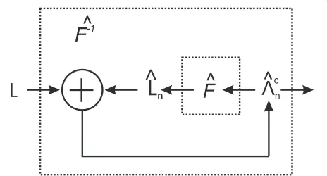
In Section 2.5 we derived two algorithms that can esti-mate a sample eigenvalue density convolved with a Cauchy density corresponding to a set of population eigenval-ues. In this section we derive a feedback method which uses the methods from Section 2.5 to correct population eigenvalue estimates.

Figure 5Schematic representation of a feedback correction.In each iteration the sample eigenvalues corresponding to the current estimate of the population eigenvalues are calculated. The estimate of the population eigenvalues is updated by comparing these sample eigenvalues with the measured eigenvalues.

But as noted in Section 2.5, we do not actually estimate the sample eigenvalues, but the convoluted sample eigen-value density gˆy(l). We therefore convolve the empirical distribution of the measured sample eigenvalue set with the Cauchy density, resulting ingy(l), and compare these two densities.

In order to derive a feedback algorithm which always converges, the best solution is to compare the distribu-tion funcdistribu-tions instead of density funcdistribu-tions. However, this requires numerical integration ofgˆy(l)which results in a large amplification of the errors in the tails of the density. Besides using densities instead of the distributions, the influence of the tail errors can be reduced even more, by considering the Kullback Leibler divergence as a measure of similarity betweengˆy(l)andgy(l)as

where we use the natural logarithm for log.

Due to numerical integration problems, the negative parts of the integral can be over estimated, resulting in a negative cost value. We therefore squared the logarithm resulting in the following cost function:

Kgy,gˆy

This is still a valid cost function: it is still 0 if and only if gy(l)= ˆgy(l)and larger than 0 for any mismatch in distri-butions. Furthermore, the focus on the tails is still reduced since lima↓0alog2a_b =0. Note also that we chosegy(l)as denominator since it is never zero fory> 0, because the Cauchy convolution kernel is never zero ify>0.

If the cost function exceeds a preset threshold, the pop-ulation eigenvalue estimates need to be adjusted. We use descending gradient to find a better estimate. To do the adjustments we need to find an expression for the gradient

∂K

The feedback correction thus created is represented schematically in Figure 6. A clear advantage of this algo-rithm is that the end result is not a density description but a set of population eigenvalues. Another advantage is that the smoothness factor is incorporated without need-ing to deconvolute the output. The last advantage is that the correction corrects all zero-valued sample eigenvalues to the same value, which is a good property as explained in Section 2.7.

2.6.3 Maintaining order among eigenvalues

For most of the methods presented in the previous sections, it is necessary that the eigenvalues are sorted in order of value and that they keep this order during updat-ing. If the order is not maintained, one of the problems that may occur is oscillation:λ˜k may switch places with

˜

λk+1in one iteration and switch back to the next iteration. Other eigenvalue correction methods had the same prob-lem. Therefore, Stein presented an algorithm to ensure order preservation during eigenvalue updating [28]. We used an isotonic tree algorithm for this purpose, described

in [10], which has several advantages over the algorithm of Stein.

2.7 Correction of the null space

A problem in eigenvalue correction occurs in underdeter-mined cases, which are characterized byNbeing smaller thanp. In this case the data matrix has a zero space and p−N+1 sample eigenvalues are necessarily zero, so the correction tries to estimateppopulation eigenvalues from N−1 non-zero sample eigenvalues.

A related effect of underdetermination is that the sam-ple eigenvectors in the null space form a random orthog-onal basis. Without additiorthog-onal information, correction of the zero-valued sample eigenvalues with varying values results in randomness in the correction. This suggests that for correction all zero-valued sample eigenvalues should be given an equal value.

A more theoretically sound argument for such a cor-rection is based on the maximum entropy theorem (see [1]). The maximum entropy method states that if there are multiple solutions to a problem and all available infor-mation has been used to narrow the selection, the best solution is the one with the highest entropy. The entropy of a multivariate normal distributed random variable is given by

1 2ln

(2πe)p||. (19)

This entropy is maximized if the determinant is maxi-mized, which is the product of the eigenvalues. With the constraint that the sum of the eigenvalues remains con-stant, the maximum of the product is achieved when all eigenvalues are equal. This is thus the maximum entropy solution.

3 Experimental validation

In the following sections we present three experiments: In the first experiment we illustrate some of the character-istics of the population eigenvalue to sample eigenvalue methods. In the second experiment we compare the per-formance of the fixed point eigenvalue correction method with an implementation we made of a state-of-the-art correction method by Karoui and a bootstrap correction method. In the third experiment we apply the correction method in a verification experiment, with a configuration often encountered in face recognition: a high number of samples with high dimensionality, where the number of samples is smaller than the dimensionality of the samples.

3.1 Population to sample eigenvalue results

In Section 2.5 we derived two algorithms to find the sample eigenvalue distribution given a set of population eigenvalues: a polynomial algorithm (Section 2.5.1) and

a fixed point algorithm (Section 2.5.2). We noted two characteristics of the methods: the polynomial algorithm will have problems if the number of eigenvalue clusters increases, and the fixed point method will require more iterations before convergence occurs if the smoothness factor is decreased.

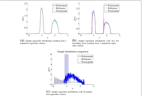
To demonstrate these characteristics we estimated the sample eigenvalue densities in three different settings: First we estimate the sample eigenvalue density of belong-ing to a population eigenvalue set with half of the eigen-values equal to 1 and the other half equal to 2, with the ratio between the dimensionality of the samples and the number of samples equal to 0.01 and with a smoothness factory(Equation 7) of 0.01 as well. In the second experiment we lower the smoothness factor to 10−5. In the third experiment we set the smoothness factor back to 0.01, but the population eigenvalue set is divided in 20 clusters uniformly distributed between 0.1 and 2.

A reference density is obtained as follows: First a syn-thetic data set is generated with the same parameters as in the experiments described. Then the sample eigenvalues of synthetic data are calculated. The corresponding empir-ical density function is then convolved with a Cauchy kernel with the same width as the smoothness factor.

Figure 7a shows the estimates of the sample eigen-value distribution for the first setting. All three estimates are very alike, only the reference estimate shows some local variations due to the use of a limited number of samples.

Figure 7b shows that when the smoothness factor is decreased, the fixed point algorithm has not con-verged on all positions if the number of iterations is kept the same. After increasing the number of iter-ations, the fixed point algorithm converged on all points again (not shown). Note that the reference dis-tribution is still convolved with a Cauchy kernel of width 0.01 so variations due to local details are kept small.

If the number of eigenvalue clusters is increased, the roots of the polynomial method become unstable and the estimation fails as shown in Figure 7c. The fixed point method is still accurate.

3.2 Sample to population eigenvalue results

As noted earlier, the more common problem is how to get from the measured sample eigenvalues an estimate of the population eigenvalues. Two methods to solve this problem were described in Section 2.6: a direct estimation method and a fixed point feedback loop method.

3.2.1 Direct estimation results

0 1 2 3 0

0.5 1 1.5 2 2.5

x

g(x)

Polynomial Reference Fixed point

(a)

0 1 2 3

0 0.5 1 1.5 2 2.5 3

x

g(x)

Polynomial Reference Fixed point

(b)

0 1 2 3

0 1 2 3 4 5 6

x

g(x)

Sample distribution comparison

Polynomial Reference Fixed point

(c)

Figure 7Sample eigenvalue density predictions based on population eigenvalues.(a) Sample eigenvalue distributions resulting from two population eigenvalue clusters. (b) Sample eigenvalue distributions with very low smoothing factor resulting from two population eigenvalue clusters. (c) Sample eigenvalue distributions with 20 population eigenvalue clusters.

estimate of the population eigenvalue density convolved with the Cauchy kernel instead of the population eigen-values. Because the Cauchy kernel has infinite variance, this poses the problem that the spread in population eigenvalues keeps increasing with an increasing number of eigenvalues. The smaller eigenvalues eventually even end up with values below zero. Because of this flaw, we did no further experiments.

3.2.2 Fixed point correction results

The second method is based on using the fixed point algorithm in Section 2.5.2 in a feedback loop as described in Section 2.6.2. In [10] we compared an eigenvalue correction method based on bootstrapping with our implementation of the method developed by Karoui. In the next experiment we repeat the comparison but we also include the iterative feedback algorithm.

The experimental set-up is as follows: Synthetic data is generated by drawing N samples from N(0,D), ap -variate normal distribution with zero mean and with diagonal matrix D as covariance matrix. From the data

the sample eigenvalues are determined and afterwards these sample eigenvalues are corrected with the three correction methods.

An accuracy score is assigned to each correction result by measuring the Levy distance between the empirical dis-tributions of the sample eigenvalues and the population eigenvalues and dividing this distance by the Levy distance between the empirical distributions of the corrections and the population eigenvalues:

score= dL(H,G) dL

H,Hˆ

(20)

where the Levy distancedLbetween distributionsFandG is given by

dL(F,G)=inf{ ≥0 :F(x− )− ≤

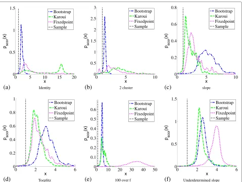
We used the Levy distance to make the experiments comparable with the experiments in [7]. But, as we showed in [10], the levy distance has several disadvan-tages, one being that the distance measure is not scale independent.

We tested six different parameter settings. In the first five only the distribution of the population eigenvalues vary. We keep the number of dimensionspfixed at 100 and the number of samplesN fixed at 500. In the last experiment, we changed N to 201 and p to 600. The settings for the population eigenvalues are given in Table 1 Experiments 1, 2, and 4 are repetitions of the experi-ments done by Karoui. We added experiment 5 because a 100 over f model is a common model for eigenvalues estimated from facial data (see [29-31] ), even though its limiting distribution is 0 for the (GSA) limit. Another characteristic of facial data is that these are underdeter-mined. The performance of the correction methods under such conditions is measured by experiment 6. To com-pare these performances with the performance if there are more samples than dimensions, experiment 3 is intro-duced.

Figure 8 gives the densities derived from the histograms of the accuracy scores, where the best method is the method that has most of its density on the right. In the identity experiment the fixed point does a reasonable job although Karoui quite frequently has better scores. In the two cluster case, Karoui is only slightly better. In the slope configuration, fixed point outperforms Karoui, but then the bootstrap method has significantly better results. In the Toeplitz case, fixed point is only slightly better than Karoui, but again the bootstrap method outperforms both methods.

So in the experiment set-ups by Karoui, the fixed point correction does not excel, but it always performs rea-sonably. However, in the last two experiments which are based on real-life settings, the results are different: in both the 100 over f configuration and the underdetermined

Table 1 The population eigenvalues per experiment

Experiment Description

1 λk=1 Identity

2 λk=1|k=1. . .50 2 Cluster λk=2|k=51. . .100

3 λk=1+k/100 Slope

4 Eigenvalues of Toeplitz matrix Toeplitz

5 λk=100/k 100 over f

6 λk=1+k/600 Underdetermined slope

The first column indicates in which experiment the eigenvalue set is used. The second column describes the eigenvalues in the set. The last column gives the name used in the text to indicate the set.

slope configuration, the fixed point method outperforms both methods clearly.

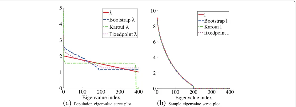
In Figure 9 we show an example repetition of the under-determined slope experiment. Figure 9a gives the scree plots of the population eigenvalue estimates, showing sig-nificant differences between estimates, and none of the estimates matches closely with the real population eigen-values. We estimated the sample eigenvalues belonging to population eigenvalue estimates and show them in Figure 9b. Despite the differences in population eigenval-ues, the sample eigenvalues seem almost identical. This suggest that the configuration is underdetermined: mul-tiple population eigenvalue sets lead to the same sample eigenvalue set. This hypothesis is further supported by Appendix 4, which shows that if the dimensionality of the samples continues to increase, in the limitation that only the mean of the population eigenvalues influences the sample eigenvalue distribution, all other characteristics are lost.

Furthermore, our implementation of the Karoui cor-rection shows that several population eigenvalues are estimated as zero valued. This becomes problematic if the training results are used, for example, for likelihood estimates.

3.3 Correction applied in verification experiments

As indicated in the previous section, bias correction can be used to improve likelihood estimates. In biometrics, a common approach to make automated verification deci-sions (that is, reject or accept the claim that a person has a certain identity based on a comparison of some measured characteristics with a template) is to model both the variations between samples coming from differ-ent persons and the variations between samples coming from the same person with normal distributions. The parameters of these distributions are estimated from a set of examples, the training set. For many biometric modalities the number of samples available for train-ing is in the same order as the dimensionality of these samples.

To show that bias reduction can, at least in theory, improve verification performance, we did a verification experiment with synthetic data, where the parameters of the distributions from which the synthetic samples are drawn have been set to the estimates obtained from facial image data. The dimensionalitypof the facial data sam-ples and the synthetic data is 8,762. The training set contained 7,047 samples of 400 individuals.

0 5 10 15 20

Figure 8Performance histograms of several correction methods.Histograms of the Levy distance ratio between the sample eigenvalue distribution and the estimates of the population eigenvalue distributions.

matrix, which cannot be done if some of the eigenvalues are zero.

The bootstrap algorithm requires usually at least 25 iterations to converge, which results in a run time of several days for the values of p and N in the experi-mental system. This run time is unacceptable in most applications.

In verification there are two kinds of claims: genuine claims, where the claimed identity is indeed the real identity of the person, and impostor claims, where the claimed identity is not the real identity of the person. In our experiment we calculated for each claim a log like-lihood ratio score, which is the logarithm of the ratio of the likelihood score that the claim is genuine over the likelihood that the claim is an impostor claim. In Figure 10 we show the score histograms achieved by applying classical principal component analysis (PCA) dimension reduction as bias correction (Figure 10a) and by applying the fixed point algorithm (Figure 10b) as bias correction.

The results show that the classical PCA reduction method will already result in highly separable likelihood scores (Figure 10a); the distance between the two clus-ters has increased considerably when using the fixed point eigenvalue correction (Figure 10b).

We also attempted to do correction in an experiment with real face data. However, we found that correction actually decreases the verification performance. This can be explained with the error in the data model we use as we reported in [31]. The smaller eigenvalues are particularly affected by the modeling error. Since eigenvalue correc-tion will increase these smaller eigenvalues, it can explain why the performance actually decreases.

4 Conclusions

0 100 200 300 400 0

1 2 3 4 5

Eigenvalue index

λ

Bootstrapλ Karouiλ Fixedpointλ

(a)

0 100 200 300 400

0 2 4 6 8 10

Eigenvalue index l

Bootstrap l Karoui l fixedpoint l

(b)

Figure 9Example of a repetition with the underdetermined slope configuration.(a) Population eigenvalue scree plot. (b) Sample eigenvalue scree plot.

between the sample eigenvalue distribution and the sam-ple eigenvalue distribution for the cases that both the number of samples and their dimensionality are infinite, so using the (MP) equation to remove the bias in practical problems is not straightforward.

To solve this problem, we showed that by setting{z} either small or large in the (MP) equation, we can focus more on local details or global characteristics of the involved eigenvalue distributions, where we assumed that global characteristics converge for much lower pandN values, andpandNonly have to close to infinite if we are interested at very local characteristics. From these obser-vations we derived methods, one of which is new to our knowledge, for estimating the sample eigenvalue density for a given set of population eigenvalues. The most impor-tant application of these methods is in a feedback algo-rithm which estimates the population eigenvalues from sample eigenvalues.

In the feedback algorithm, the value of {z} deter-mines how the estimated sample eigenvalue density and

the empirical distribution of the measured sample eigen-values are smoothed before they are compared. Increas-ing {z} when both p and N are limited reduces the influence of statistical noise in the correction at the price of loosing details of the population eigenvalue density.

We showed that the feedback algorithm particularly outperforms other methods in the underdetermined con-figurations and concon-figurations where individual eigenval-ues are of importance, such as the set described by a 1 over f distribution, which is often encountered in biometrics. In a verification experiment, application of the feedback method results in a large increase of the distance between impostor and genuine scores. The difference between the synthetic scores of the classical PCA method and the scores achieved using real data suggests that the bias in the sample eigenvalues is not the only problem in face data though. Eigenvalue correction can actually increase the effect of modeling errors and therefore result in a decreased performance.

-800 -600 -400 -200 0 200

0 0.01 0.02 0.03 0.04 0.05 0.06

PCA correction scores

Imposter Genuine

(a)

-10000 -5000 0 5000

0 1 2 3 4x 10

-3Fixed point correction scores Genuine

Imposter

(b)

If the distribution of the data is (approximately) known, finite sample size eigenvalue distributions have been determined for several data distributions. These solution can take advantage of details lost in the limit analy-sis used for deriving the (MP) equation. The transition point when one approach outperforms the other is at this time difficult to determine, partially because convergence behavior is still a topic of study for the (MP) equation. A disadvantage for distribution-specific approaches is that unless prior knowledge is available, the data distribution should be tested. For some of these tests it has already been shown that their accuracy is negatively affected by increased dimensionality of the data. In previous stud-ies we already saw that for large dimensionality, (GSA)-based methods outperformed a data distribution-specific method. How the relation is with other distribution spe-cific methods is however still an open question.

Appendix 1

Proof influence of parts of the distribution on the Stieltjes transform

In this section we prove that the Stieltjes transform atzis influenced mostly by changes in the density close to{z}. Assume we are going to move a part of the density ofG(l) around positionl1with weightβ. We assume the part we move to be small enough soG(l)can be written asG(l)= (1−β)G(l)˜ +βu(l−l1). The Stieltjes transformmG(z) can be written as

mG(z)=

The derivative ofmG(z)with respect tol1, normalized forβis then given by

with its maximum value, we get

so the norm of the derivative is a function which has a maximum at {z} = l1 and its width is proportional to{z}.

The sample eigenvalue density is solely determined by the imaginary part of the Stieltjes transform (Equation 7). The width of the function of the imaginary part of the derivative is also proportional to {z}, although its extrema are not exactly at{z} =l1:

Proof result integration along circle stays within circle

Note that the integrals in Equations 4 and 6 can be rewrit-ten to the form

dF(a(r))

r−ıq (29)

whereris a real variable,qis a real constant, Fis a dis-tribution function andais a functionR → R. We now prove that the result of the integrals stays within the circle described by(r−ıq)−1, by showing that the norm of the result minus the center of the circle can never exceed the radius of the circle.

Proof fixed point in fixed point solution

In this section we prove that the function in Equation 10 has a fixed point. According to the Banach fixed point theorem, we need to show that d(An+1 −Bn+1) ≤ q ·

d(An−Bn)holds for any two pointsAandB, whereq<1 [24]. We begin by evaluating the norm of the difference between both points of iterationn+1:

=γ |An−Bn|

From this we can derive an expression for the ratio which should be between 0 and 1 according to the theorem

Note that the minimum norm of An is determined by 1

max|v∞(z)| = {z}, so the minimum norm ofAn is equal to the smoothness factor. Therefore, setting the smooth-ness factor arbitrarily large will result in an arbitrarily low ratio of Equation 36, guaranteeing convergence after some threshold in the value of the smoothness factor.

A minimum value of the smoothness factor can be derived after which convergence is guaranteed. Assume that 0< γ < 1. Then if both maximums in Equation 38 get close to 1, the ratio of Equation 36 becomes smaller than 1.

We will focus on the first ratio, since the argument on the second ratio is similar. Given|λ+An| > λ, the ratio

max_λ+λ_An is smaller than 1, therefore convergence is guaranteed. Setting the smoothness factor larger than 2λmax, where 2λmax = maxλk, will result in a minimum norm ofAnof 2λmax. This results in a ratio lower than 1, guaranteeing convergence of the algorithm. There is even a lower setting for the smoothness factor sinceAnattains its minimum norm when it is purely imaginary. In that case, the norm has an upper limit of√1

5.

Appendix 4

Underdetermination in high-dimensional problems

In the experiments we suggest that if the number of samples N is below the dimensionality of the samples p, the correction of the sample eigenvalues is an under-determined problem. In the following section we prove that if γ → ∞, all characteristics of the population eigenvalue distribution are lost except for its mean, show-ing that in that limit the sample eigenvalue correction is indeed a severely underdetermined problem. Because H(λ) describes the population eigenvalues, H(λ) = 0∀λ ≤ 0. We also assume the eigenvalues have a supre-mumλsup, soH(λ)=0∀λ > λsup.

We start with proving thatO(v∞(z))=Oγ−1. We first show thatO(v∞(z))=O(γa), witha>0 leads to a contradiction. Firstly, note thatO_v 1

∞(z) determine the sample eigenvalue distribution ifγ → ∞,

lim

So in the limit the Stieltjes transformv(z)converges to v(z)= 1

γλ¯−z

Competing interests

The authors declare that they have no competing interests.

Received: 20 May 2012 Accepted: 21 May 2013 Published: 12 June 2013

References

1. E Jaynes, On the rationale of maximum entropy methods. Proc. IEEE, Spec Issue on Spectral Estimation.70, 939–952 (1982)

2. J Särelä, R Vigário, Overlearning in marginal distribution-based ICA: analysis and solutions. J. Mach. Learn. Res.4(7–8), 1447–1469 (2004) 3. ZD Bai, Methodologies in spectral analysis of large dimensional random

matrices, a review. Statistica Sinica.9, 611–677 (1999) 4. A Hendrikse, R Veldhuis, L Spreeuwers, inProceedings of the 30th

Symposium on Information Theory in the Benelux. Improved variance estimation along sample eigenvectors (Werkgemeenschap voor Informatie- en Communicatietheorie Eindhoven, 28–29 May 2009), pp. 25–32

5. ZD Bai, H Saranadasa, Effect of high dimension: by an example of a two sample problem. Statistica Sinica.6, 311–329 (1996)

6. PJ Phillips, PJ Flynn, T Scruggs, KW Bowyer, J Chang, K Hoffman, J Marques, J Min, W Worek, inCVPR ’05: Proceedings of the 2005 IEEE Computer Society Conference on Computer Vision and Pattern Recognition (CVPR’05), vol. 1. Overview of the face recognition grand challenge (Washington, DC, 2005), pp. 947–954

7. N El Karoui, Spectrum estimation for large dimensional covariance matrices using random matrix theory. Ann. Stat.36(6), 2757–2790 (2008) 8. VA Marˇcenko, LA Pastur, Distribution of eigenvalues for some sets of

random matrices. Math. USSR - Sbornik.1(4), 457–483 (1967) 9. JW Silverstein, Strong convergence of the empirical distribution of

eigenvalues of large dimensional random matrices. J. Multivar. Anal. 55(2), 331–339 (1995)

10. AJ Hendrikse, LJ Spreeuwers, RNJ Veldhuis, inICDM ’09. A bootstrap approach to eigenvalue correction (IEEE Computer Society Press Miami, Florida, 2009), pp. 818–823

11. V Girko,Theory of Random Determinants. (Kluwer, Boston, 1990) 12. AM Tulino, S Verdú,Random Matrix Theory and Wireless Communications.

(Now Publishers Inc., Norwell, 2004)

13. A Maaref, S Aissa, Eigenvalue distributions of Wishart-type random matrices with application to the performance analysis of MIMO MRC systems. Trans. Wireless. Comm.6(7), 2678–2689 (2007). [http://dx.doi. org/10.1109/TWC.2007.05990]

14. F Neeser, J Massey, Proper complex random processes with applications to information theory. IEEE Trans Inf. Theory.39(4), 1293–302 (1993) 15. TW Anderson,An Introduction to Multivariate Statistical Analysis. Wiley Series

in Probability and Mathematical Statistics, 2nd edn. (Wiley, New York, 1984) 16. RJ Muirhead,Aspects of multivariate statistical theory. (Wiley Series in

Probability and Mathematical Statistics. (Wiley, New York, 1982) 17. AJ Hendrikse, RNJ Veldhuis, LJ Spreeuwers, AM Bazen, inAdvances in

Biometrics, Alghero, Italy, Volume 5558/2009 of Lecture Notes in Computer Science. Analysis of eigenvalue correction applied to biometrics (Springer Verlag Berlin / Heidelberg, 2009), pp. 189–198

18. EB Saff, AD Snider,Fundamentals of Complex Analysis with Applications to Engineering, Science, and Mathematics, 3rd edn. (Pearson Education, Upper Saddle River, 2003)

19. S Tsai, Characterization of Stieltjes transforms 2000. http://etd.lib.nsysu.

edu.tw/ETD-db/ETD-search/getfile?URN=etd-0626100-163925&filename=qq.pdf&ei=0py3Uci1Huq90QWsi4DIBA&usg= AFQjCNEE1lvVNJAYZ59IjPIFTQyS7KpNdA, Accessed 11 June 2013 20. NR Rao, A Edelman, The polynomial method for random matrices.

Foundations Comput Math.8, 649–702 (2008). [http://dl.acm.org/citation. cfm?id=1474542.1474546]

21. JH Wilkinson,Rounding errors in algebraic processes. Notes on applied science. (Prentice Hall, Englewood Cliffs, 1963)

22. L Reichel, On polynomial approximation in the complex plane with application to conformal mapping. Comput. Math.44(170), 425–433 (1985)

23. G Sitton, S Burruns, JW Fox, S Trietel, Factoring very high degree polynomials. IEEE Signal Process Mag.20(6), 27–42 (2003)

24. VI Istr˘a¸tescu,Fixed Point Theory: An Introduction. vol. 7 of Mathematics and its Applications. (D Reidel Publishing Co, Dordrecht, 1981)

25. J Carrier, L Greengard, V Rokhlin, A fast adaptive multipole algorithm for particle simulations. SIAM J. Sci. Stat. Comput.9(4), 669–686 (1988) 26. L Greengard, V Rokhlin, A fast algorithm for particle simulations. J

Comput. Phys.73(2), 325–348 (1987). [http://dx.doi.org/10.1016/0021-9991(87)90140-9]

27. M Gu, SC Eisenstat, A divide-and-conquer algorithm for the symmetric TridiagonalEigenproblem. SIAM J. Matrix Anal. Appli.16, 172–191 (1995). [http://dx.doi.org/10.1137/S0895479892241287]

28. C Stein, Lectures on the theory of estimation of many parameters. J Math. Sci.34, 1371–1403 (1986)

29. X Jiang, B Mandal, A Kot, Eigenfeature regularization extraction in face recognition. IEEE Trans. Pattern Anal Mach. Intell.30(3), 383–394 (2008) 30. B Moghaddam, A Pentland, Probabilistic visual learning for object

representation. IEEE Trans. Pattern Anal Mach. Intell.19, 696–710 (1997) 31. AJ Hendrikse, RNJ Veldhuis, LJ Spreeuwers, inThirty-first Symposium on

Information Theory in the Benelux. The effect of position sources on estimated eigenvalues in intensity modeled data (Werkgemeenschap voor Informatie- en Communicatietheorie, Rotterdam, 11–12, May 2010), pp. 105–112

doi:10.1186/1687-6180-2013-117

Cite this article as:Hendrikse andet al.:Smooth eigenvalue correction.

EURASIP Journal on Advances in Signal Processing20132013:117.

Submit your manuscript to a

journal and benefi t from:

7Convenient online submission 7 Rigorous peer review

7Immediate publication on acceptance 7 Open access: articles freely available online 7High visibility within the fi eld

7 Retaining the copyright to your article