Full waveform moment tensor inversion by reciprocal finite difference
Green’s function
Taro Okamoto
Department of Earth and Planetary Sciences, Tokyo Institute of Technology, 2-12-1 Ookayama, Meguro, Tokyo 152-8551, Japan
(Received July 18, 2001; Revised April 6, 2002; Accepted April 9, 2002)
We study two important aspects of the waveform moment tensor inversion for the shallow earthquakes in the subduction region: the effect of the intense lateral inhomogeneity in the structure, and the strategy to invert the waveform data for the focal mechanisms. For the first aspect, using a “forward” finite difference modeling, we demonstrate that the effect of the inhomogeneity is quite large on the surface waves with a period of about 20s, and the current knowledge on the subduction region structure is practically effective in reproducing the characteristics in the observed waveforms. For the second aspect, we develop a “reciprocal” moment tensor inversion method that can generate the Green’s functions for a large quantity of source locations (19,200 in this study) in a realistic inhomogeneous structure by only three finite difference calculations per a single station. The inversion with a grid search scheme result in a reasonable source location, moment tensor and fit of the waveforms using data from only two stations. The constraint on the epicenter in the “transverse” direction is found to be somewhat weak in the case of single-station inversions, but the two-station inversion improves the constraint.
1.
Introduction
The waveform inversion of the moment tensor of the earthquakes provides important contributions to the study of tectonics and earthquake source physics. Many projects for routine determination of the moment tensor have been established and being kept for years (e.g., Dziewonski and Woodhouse, 1983; Sipkin, 1994; Kawakatsu, 1995; Pasyanoset al., 1996; Fukuyamaet al., 1998). Also, wave-form inversion is the basis of the rupture process analysis of the fault (e.g., Kikuchi and Kanamori, 1991). The cur-rent routine regional analysis usually assumes a laterally homogeneous structure in calculating the synthetic wave-forms (Green’s functions) although the actual structure is of-ten strongly laterally inhomogeneous. Such inhomogeneity has non-negligible effects especially on the surface waves such as the changes in the phase velocity (e.g., Thio and Kanamori, 1995) or the curved paths and multiple paths (e.g., Tanimoto, 1990) and can be the cause of the artificial noise in the inversion process. The most straightforward way to remove this problem is to calculate the synthetic waveforms using realistic laterally inhomogeneous structure.
In the moment tensor inversions we need at least five Green’s functions (under the commonly applied condition trace(Mi j) = 0)for each source-station pair. This implies
five “forward” simulations with five elementary source types per a single station. However, it is not enough because we usually need to search the optimum source location by the inversion procedure itself rather than to fix it in the inver-sion. Thus the number of required simulations per a single station would be up to five times as many as the number of
Copy right cThe Society of Geomagnetism and Earth, Planetary and Space Sciences (SGEPSS); The Seismological Society of Japan; The Volcanological Society of Japan; The Geodetic Society of Japan; The Japanese Society for Planetary Sciences.
potential source locations if we performed forward simula-tions for every potential sources. This behavior makes the inversion very impractical as the simulation of seismic waves in inhomogeneous structure is still quite numerically inten-sive.
A more practical strategy is the use of “reciprocal” mod-eling (e.g., Okamoto, 1994a, b): based on the reciprocal the-orem, a single force is applied at the station location, and the response strain recorded at the source location is convolved with the moment tensor to generate the seismic displacement at the station location. The strain time functions for a number of arbitrary source locations can be stored in a single simula-tion if we use methods like finite difference or finite element. Thus a large number of Green’s functions can be calculated by only three simulations (for three components) per a single station, which makes the inversion procedure very feasible.
In this short paper we demonstrate the importance of the lateral inhomogeneity in generating the synthetic wave-forms, and show the results of the reciprocal moment tensor inversions with a grid search scheme for the optimum source location and focal mechanism.
2.
Data and Forward Modeling
We select an event in the Japan trench on 23 Feb. 1995 05:01 UTC (MW6.2) as a typical example of the shallow
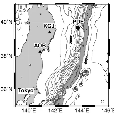
event in the subduction region where the lateral inhomogene-ity is very strong. The broadband waveform data at two sta-tions (KGJ and AOB: Fig. 1) maintained by Research Center for Prediction of Earthquakes and Volcanic Eruptions, Grad-uate School of Science, Tohoku University are downloaded using the GOPHER system installed in Earthquake Research Institute, University of Tokyo.
We assume a model structure for the Japan trench based on the results of the seismic refraction experiments (Murauchi
140˚E
142˚E
144˚E
146˚E
36˚N
38˚N
40˚N
6000 6000 4000
2000
PDE
KGJ
AOB
Tokyo
Fig. 1. The PDE epicenter of the event (solid circle) and the stations (solid triangles). The contour interval in the oceanic region is 500 m. Shaded area (deeper than 6500 m) in the ocean indicates the trench axis.
and Ludwig, 1980; Suyehiro et al., 1986: see Fig. 2 and Table 1). In order to reduce the required computational resources, we use a “2.5D” finite difference method (the structure is 2D but the wavefield is full-3D and the spatio-wavenumber mixed domain is used for calculation: see e.g., Okamoto 1994b; Furumura and Takenaka, 1996). The ma-terial properties are assumed to be identical with respect to the trench-parallel axis because of the nearly 2D topography of the studied area. We also assume homogeneous mantles (separated by the oceanic crust) in order to reduce numer-ical computations although the modeled surface waves can penetrate into the mantle.
Before going to the inversion analysis, it is important to see the effect of the laterally inhomogeneous structure by employing forward modelings. We apply a point source at the PDE epicenter (39.66N, 143.69E) with a depth of 15 km, the best double couple mechanism of the Harvard CMT (HCMT) solution (strike 190◦, dip 13◦, slip 81◦), a seismic moment of 2.15×10¹⁸Nm, and a Gaussian moment
rate function f(t) = exp(−αt2)whereα = 0.1. A 10–
100 s bandpass filter is applied to both of the synthetic and the observed waveforms, but frequency components around 0.05 Hz (period of 20 s) dominate the waveforms as shown in Fig. 3. Also we employ a simulation for a flat, laterally homogeneous structure. We simply adopt the crustal model under the northern Japan with an addition of a thin surface layer (Table 2).
The synthetics for the realistic 2.5D structure show re-markable resemblance to the observed data (Fig. 3): the dis-persive wave train in the observed surface waves are well reproduced in these synthetics. On the other hand, the syn-thetics for the assumed flat structure show relatively low dis-persive behavior and they do not show good resemblance to the data.
It is often possible to reproduce the effect of
inhomoge-VERT.EXAG. 2.0
0km
0km 40km
300km
1.5
2.0
4.5
5.8
6.5
7.8
6.7
8.1
2.0
Fig. 2. The vertical cross section of the assumed 2.5D (semi-3D) structure for FDM calculations, which is taken to be perpendicular to the trench axis. The P-wave velocities for each layer in km/s are indicated. For other material parameters see Table 1. The FDM parameters are: hor-izontal (trench-normal) and vertical grid spacings of 1 km, minimum wavelength of 5 km with respect to trench-parallel axis, size of 700 km (trench-normal)×740 km (trench-parallel)×300 km (vertical), 121 wavenumbers, time steps of 3000 (168 s). The program requires about 212 MB (mega bytes) of memory, and about 34 hours for calculation of one component on Compaq Alpha based machine (21264/666 MHz).
Table 1. Structural parameters for the 2.5D (semi-3D) realistic model. The parameters in a vertical cross section (Fig. 2) are listed. VP: P-wave
velocity in km/s.VS:S-wave velocity in km/s.ρ: density in g/cm3.
layer VP VS ρ
sea water 1.5 0.0 1.0
sediment (1) 2.0 1.0 2.0
sediment (2) 4.5 2.6 2.5
upper crust 5.8 3.35 2.6
lower crust 6.5 3.75 2.8
mantle (1) 7.8 4.5 3.2
oceanic crust 6.7 3.87 2.9
mantle (2) 8.1 4.68 3.3
Table 2. Structural parameters for the flat layered model. “d” denotes layer thickness in km.
layer VP VS ρ d
sediment 4.5 2.6 2.5 2.0
upper crust 5.8 3.35 2.6 8.0
lower crust 6.7 3.87 2.9 15.0
mantle 8.1 4.68 3.3 ∞
neous structure on the surface waves by adopting a 1D (flat-layered) structure whose phase and group velocities are ad-justed to the observational ones averaged over the path, pro-vided the inhomogeneities are not so strong. (In that sense above 1D model is not adjusted for the realistic surface wave velocities.) Detailed study of the limit and/or the applicabil-ity of 1D structure is beyond the scope of this short paper, but we here indicate another aspect of the structural effect. Figure 4 shows the synthetic waveforms of a forward mod-eling with the same parameters as above but for anisotropic
P
Fig. 3. The observed and the “forward” synthetic displacement for sta-tion KGJ. “2.5D” denotes the synthetics for the realistic 2.5D structure, and “FLAT” for the flat layered structure. The number attached to the observed waves are maximum amplitudes in mm.
140s
TransverseRadial Vertical
Fig. 4. The synthetic displacement for an isotropic (explosive) source and for station AOB. The FDM region (900 km×1140 km×400 km) is a little larger than that for other calculations. Arrow indicates the onset of surface waves.
result of Rayleigh to Love wave conversion due to the inho-mogeneous structure. Such effect cannot be reproduced by any flat-layered model.
These examples show the importance of the laterally in-homogeneous structure in modeling the waveforms, and also show the current knowledge on the structure is practically ef-fective in modeling the waveforms of period around 20 sec-onds. Note that we did not “tune” the structural model in
calculating these results but we simply adopted the results of the seismic experiments. However, there still are slight misfits to the data, which may be corrected by searching the optimum source location and the focal mechanism (moment tensor). This is demonstrated in the next section.
3.
Reciprocal Inversion and Results
Based on the reciprocal theorem, we store the strain com-ponents at the grids in a box-shaped region (195 km×195 km in horizontal and 22 km in vertical) with 5 km horizontal and 2 km vertical spacings. Thus the potential source loca-tions amounts to 19,200. Our strategy is to perform wave-form moment tensor inversion for each of these 19,200 grids and to apply a grid search scheme in order to find the opti-mum source location. The residual minimized in the wave-form inversion is:
whereNstadenotes the number of stations,T the time
dura-tion (110 s from the P-wave arrival), Oi k(t)andCi k(t)the
observed and calculatedk-th component of the displacement ati-th station, respectively, andw(t)the weighting function. We setw(t)=2 for the first 25 s for KGJ and 34 s for AOB, andw(t) = 1 for other portion in order to compensate the small amplitude of the body waves. In order to avoid numer-ical dispersions, we use a smooth Gaussian source function which is slightly broader than the observed first pulse. Be-cause the onset of the synthetic pulse is very emergent (i.e., the amplitude gradually increases), the synthetics are slightly shifted by minimizing the residualS. This effectively adjust the overall arrival of the synthetic P-wave pulse but its very onset cannot be adjusted to the observation under current nu-merical parameters. Therefore, we do not discuss the source time (or the centroid time). We employ two single-station in-versions (denoted by “KJG” and “AOB” for each station) and one multi(two)-station inversion (denoted by “KGJ+AOB”).
KGJ
AOB
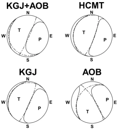
The HCMT and the moment tensor solutions have similar characteristics except for the single-station solution for AOB (Fig. 5): the principal axes (P- andT-axes) have almost the same directions, and the polarities are nearly the same. Also, the strikes of the steeper nodal planes of the best double couples have nearly NNE-SSW trends consistent with the geometry of the subduction. The strikes of the shallower nodal plane are not constrained well in the present study.
The slightly improper mechanism for AOB (single-station) is due to the weak constraint on the source location in the “transverse” direction. This is illustrated in Fig. 6 which plots the horizontal cross sections of the residuals sliced through the optimum source depths. The inversion for KGJ (top) shows a distinct, prolonged trough
extend-KGJ
AOB MIN=0.39DEP= 9.0km 100km
KGJ
AOB
KGJ+AOB
KGJ
AOB MIN=0.35DEP=15.0km 100km
KGJ
AOB MIN=0.55DEP=15.0km 100km
0.5
1.0
1.0
0.5
1.0
1.0
0.6
0.6
0.6
1.0
1.0
Fig. 6. The horizontal cross sections of the residuals sliced through the optimum source depth. The vertical line of the figure is parallel to the trench axis and the horizontal line is normal to the trench axis. The waveform inversions are done for points in the inner box. The contour interval is 0.1. Solid circles indicate the optimum points for the source locations. The PDE epicenter (cross) and the two stations (solid triangles) are also projected for reference. The area with residuals smaller than 0.6 are gray-shaded in middle figure to indicate the region of local minima.
ing nearly along an arc whose center of curvature is the sta-tion KGJ. This indicates a weak constraint on the epicentral parameters in the transverse direction (along the arc). The single-station inversion for AOB (middle) also shows simi-lar feature that the residual trough align along an arc with a center roughly being the station. However, the pattern is more complex and there are many local minima. The solu-tion falls into one of these local minima, which results in a slightly improper mechanism. Also, effects due to the devi-ation of the actual 3D structure from the assumed 2D model must be larger for AOB, which decrease the accuracy of the synthetics and may be partially responsible for the improper mechanism.
Despite of these uncertainties, the result of the two-station inversion (bottom) shows a single, relatively well defined global minimum. The trough in the residual pattern be-comes more compact although it still have some prolonged feature. Note that the best point is not a simple average of the best points of the two single-station inversions, but it occurs approximately at the intersection point of the two arc-like troughs shown in the single-station inversion results. Be-cause both the troughs for KGJ and AOB run through the reasonable point, the two-station inversion yields a reason-able solution (see also Fig. 7).
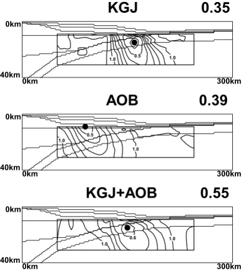
Figure 7 shows the vertical cross sections of the residual distributions plotted on the assumed structure through the optimum point. The single-station inversion for KGJ (top) results in a fairly well constrained global minimum for the source location. The optimum location is also reasonable be-cause this event is an interplate thrusting one. This shows a proper constraints on the source position in the “radial” and
0km
0km 40km
300km 0km
0km 40km
300km 0km
0km 40km
300km
KGJ+AOB
AOB
KGJ
0.35
0.39
0.55
0.5 1.01.0
1.0
1.0 1.0
0.5
1.0 0.6
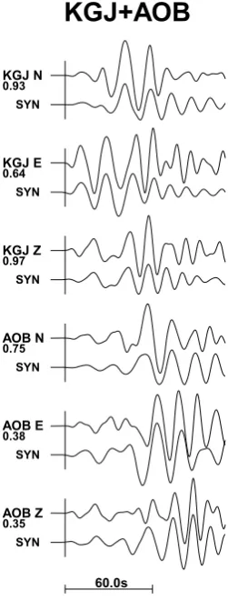
KGJ+AOB
Fig. 8. The observed and synthetic waveforms calculated by the two-station inversion. The upper trace in each component is the observed one. Vertical lines indicate the onsets of theP-waves. Maximum amplitudes in mm are also indicated.
vertical direction. The solution of the single-station inver-sion for AOB (middle) falls into a local minimum discussed above so that the position is not reasonable for this type of event. The result of the two-station inversion (bottom) indi-cate a well defined minimum at a reasonable position. Thus, as well as the source depth, the source location is well con-strained both in transverse and radial directions in the two-station inversion.
Figure 8 shows the observed and the synthetic waveforms for the two-staion inversion. The dispersive feature in the surface wave is still clearly preserved and the first motions (i.e., polarity of the P-wave) of all the synthetics are consis-tent with the data.
4.
Discussion and Conclusion
The focal depths of the events of the seismic activity in northern Japan trench have been precisely determined by land-side observations of the depth phases (i.e.,StoP con-version at the surface: Uminoet al., 1995) and by in-situ observations by the ocean bottom seismometers (Hinoet al., 1996). These reports determined the focal depths of the events in the region studied in this paper to be around 15 km with a scatter of about±5 km. The optimum depth obtained by our waveform inversion (15 km) is in good agreement with these precisely determined source depths.
Single-station inversion using the near-source seismic
recordings is sometimes inevitable as the good near-source recordings is often rare in many regions (e.g., Delouis and Legrand, 1999). There is a similar situation in the subduction region: the station coverage is often one-sided and not quite good because of the presence of the ocean where seismic stations are very rare. Even under such situations, we have demonstrated that reasonable moment tensor and source lo-cation can be estimated by the waveform inversions with the reciprocal finite difference Green’s function, provided that data from two (or more) stations are available.
We have also demonstrated the strong effect of the inho-mogeneous structure (Fig. 4) that cannot be modeled by any flat-layered model. Such effects must be considered care-fully, especially in the waveform study of the rupture pro-cess on the fault plane (e.g., Mori and Shimazaki, 1985; Nakayama and Takeo, 1997) as the location of the subevents are determined solely based on the waveform data.
The conclusions of this paper are: (1) The current knowl-edge on the subduction region structure is practically effec-tive in reproducing its large effects on the observed wave-forms. (2) An efficient “reciprocal” moment tensor inversion method is developed. (3) Reasonable moment tensors are ob-tained by the reciprocal inversion. The fit of the synthetics to the observed waveforms is also good. (4) The residual distributions indicate somewhat non-unique behavior in the estimation of the epicentral location especially for the single-station inversions. The epicentral solution for the two-single-station inversion is more stable.
Acknowledgments. The author is grateful to the staffs in Research Center for Prediction of Earthquakes and Volcanic Eruptions, Grad-uate School of Science, Tohoku University and Earthquake Re-search Institute, University of Tokyo for their online data base. The author is also grateful to Yasuhiro Yoshida, Yasumaro Kakehi and G¨oran Ekstr¨om for critically reviewing the manuscript. Discus-sions with Naoki Kobayashi were also helpful. This research is partially supported by the Grant-in-Aid for Scientific Research (C) (No. 08640527) from the Ministry of Education, Science, Sports and Culture of Japan. One of the calculations was employed in Earthquake Research Institute, University of Tokyo.
References
Delouis, B. and D. Legrand, Focal mechanism determination and identifica-tion of the fault plane of earthquakes using only one or two near-source seismic recordings,Bull. Seism. Soc. Am.,89, 1558–1574, 1999. Dziewonski, A. M. and J. H. Woodhouse, Studies of the seismic source
using normal mode theory,Proc. Enrico Fermi Sch. Phys.,85, 45–137, 1983.
Fukuyama, E., M. Ishida, D. S. Dreger, and H. Kawai, Automated seismic moment tensor determination by using on-line broadband seismic wave-forms,Zisin (J. Seism. Soc. Japan, 2nd series),51, 149–156, 1998 (in Japanese with English abstract).
Furumura, T. and H. Takenaka, 2.5-D modelling of elastic waves using the pseudospectral method,Geophys. J. Int.,124, 820–832, 1996.
Hino, R., T. Kanazawa, and A. Hasegawa, Interplate seismic activity near the northern Japan Trench deduced from ocean bottom and land-based seismic observations,Phys. Earth Planet. Inter.,93, 37–52, 1996. Kawakatsu, H., Automated near-realtime CMT inversion, Geophys. Res.
Lett.,22, 2569–2572, 1995.
Kikuchi, M. and H. Kanamori, Inversion of complex body waves—III,Bull. Seism. Soc. Am.,81, 2335–2350, 1991.
Mori, J. and K. Shimazaki, Inversion of intermediate-period Rayleigh waves for source characteristics of the 1968 Tokachi-Oki earthquake,J. Geo-phys. Res.,90, 11374–11382, 1985.
Washington, 1980.
Nakayama, W. and M. Takeo, Slip history of the 1994 Sanriku-Haruka-Oki, Japan, earthquake deduced from strong-motion data,Bull. Seism. Soc. Am.,87, 918–931, 1997.
Okamoto, T., Location of shallow subduction zone earthquake inferred from teleseismic body waveform,Bull. Seism. Soc. Am.,84, 264–268, 1994a. Okamoto, T., Teleseismic synthetics obtained from 3-D calculations in 2-D
media,Geophys. J. Int.,118, 613–622, 1994b.
Pasyanos, M. E., D. S. Dreger, and B. Romanowicz, Toward Real-Time Estimation of Regional Moment Tensors,Bull. Seism. Soc. Am., 86, 1255–1269, 1996.
Sipkin, S. A., Rapid determination of global moment-tensor solutions, Geo-phys. Res. Lett.,21, 1667–1670, 1994.
Suyehiro, K., T. Kanazawa, and H. Shimamura, Air gun-ocean bottom seismograph seismic structure across the Japan trench area, inInitial
Reports of the Deep Sea Drilling Project, edited by H. Kagami, D. E. Karig, W. T. Coulbournet al.,87, U.S. Govt. Printing Office, Washington, 1980.
Tanimoto, T., Modelling curved surface wave paths: membrane surface wave synthetics,Geophys. J. Int.,102, 89–100, 1990.
Thio, H. K. and H. Kanamori, Moment tensor inversions for local earth-quakes using surface waves recorded at TERRAscope,Bull. Seism. Soc. Am.,85, 1021–1038, 1995.
Umino, N., A. Hasegawa, and T. Matsuzawa, s P depth phase at small epicentral distances and estimated subducting plate boundary,Geophys. J. Int.,120, 356–366, 1995.