Essays on inequality and intergenerational mobility in China

(1)

The London School of Economics and Political Science

Essays on Inequality and Intergenerational

Mobility in China

Yi Fan

(2)

Declaration

I certify that the thesis I have presented for examination for the PhD degree of the London School of Economics and Political Science is solely my own work other than where I have clearly indicated that it is the work of others (in which case the extent of any work carried out jointly by me and any other person is clearly identified in it).

The copyright of this thesis rests with the author. Quotation from it is permitted, provided that full acknowledgment is made. This thesis may not be reproduced without the prior written consent of the author.

I warrant that this authorization does not, to the best of my belief, infringe the rights of any third party.

(3)

Statement of conjoint work

Chapter 2, “The Great Gatsby Curve in China: Cross-Sectional Inequality and Intergener-ational Mobility”, was jointly co-authored with Professor Junjian Yi and Professor Junsen Zhang.

This statement is to confirm that I contributed a minimum of 33% of this work. More specifically, I have carried out the empirical analyses.

Statement of use of third party for editorial help

I can confirm that my thesis was proofread by Ms. Skye Hughes, Ms. Elizabeth Storer, Ms. Jacqueline Wah, and editors at Transformat.

(4)

Acknowledgment

I am grateful to my supervisors, Robin Burgess, Guy Michaels, and Diana Weinhold, for their continued support and encouragement. Thanks for guiding me through all the ups and downs, pushing me to think hard on the topic and structure of this thesis, responding to my questions in no time at all, and encouraging me to be mentally strong and cheerful when I was completing the degree studies and searching the job market.

I am indebted to my MPhil supervisor, Junsen Zhang, at the Chinese University of Hong Kong (CUHK), for leading me into the world of economics research, and granting me access to the 2005 China mini-census and the 2002 Chinese Twins Survey. I owe appreciation to my CUHK colleague and mentor, Junjian Yi, for sharing his invaluable research experience and illuminating the detailed work for me. I have enjoyed learning from them during our joint work on the second chapter of this thesis.

Special thanks go to Gary Becker, Steven Durlauf, and James Heckman for very help-ful comments and suggestions on the second chapter of the thesis.

I thank Mayling Birney, Jean-Paul Faguet, Alan Manning, Rachel Ngai, Steve Pis-chke, and Sandra Sequeira, for their advice. I would also like to thank my PhD col-leagues and friends, Anila Ahsan, Shiyu Bo, Svetlana Bryzgalova, Benjamin Chemouni, Xiaoguang Chen, Francisco Costa, May Chu, Jonathan De Quidt, Laura Derksen, Erika Deserranno, Andy Feng, Thiemo Fetzer, Giulia Ferrari, Pei Gao, Jason Garred, Georg Graetz, Nelson A Ruiz-Guarin, Fadi Hassan, Shiyang Huang, Ivor Jones, Reka Juhasz, Kohei Kawaguchi, Andrea Lanteri, Yu-Hsiang Lei, Kun Li, Jiawei Lim, Suyu Liu, Chenyan Lu, Yiqing Lv, Ting Luo, Enrico Mallucci, Sam Marden, Eduardo Mello, Laura Munro, Oliver Pardo-Reinoso, Georgie Pearson, Joao Paulo Pessoa, Anouk Rigterink, Munir Squires, Pedro Souza, Elizabeth Storer, Eddy Tam, Maria Lopez-Uribe, Petterson Molina Vale, Maria Waldinger, Fabian Winkler, Yanyan Xiong, Xun Yan, Yang Yan, Junxiang Zhang, and Min Zhang, for constructive discussion and kind support. Comments from seminar participants at LSE, conference participants at the Royal Economic Society, Eu-ropean Economic Association, EuEu-ropean Society of Population Economics, Chinese Eco-nomic Association, IZA/World Bank conferences, and 2013 Summer School on Socioe-conomic Inequality at The University of Chicago are highly appreciated.

(5)

Abstract

This thesis consists of three essays on intragenerational and intergenerational inequal-ity. It focuses on the largest developing country, China, and examines historically and currently under-represented groups.

The first chapter, “Does Adversity Affect Long-term Consumption and Financial

Behaviour? Evidence from China’s Rustication Programme”, investigates the

long-term effects of early experiences on economic behaviour, by referring to the largest forced migration experiment in history. Focusing on the historically under-represented group of people who were sent from urban to rural areas to do manual farm work during their adolescence, I demonstrate that they behave conservatively over the long term. They spend less on housing, accumulate more savings and insurance, and invest less in risky assets. One mechanism for the conservative behaviour lies in the habits formed during adversity. My study sheds light on how a policy, experienced especially in the early stage of life, influences a generation over the long term.

In addition to inequality, the second and the third chapters examine intergenerational mobility. The second chapter, “The Great Gatsby Curve in China: Cross-Sectional

Inequality and Intergenerational Mobility”, estimates the extent of the decline in

inter-generational mobility in income and education during China’s economic transition. The decline is more evident for the currently under-represented groups: females, and resi-dents of rural areas and the western regions. To correlate intergenerational mobility with cross-sectional inequality, a Great Gatsby Curve with a negative slope is presented, and related institutional factors are discussed. This chapter is written jointly with Junjian Yi and Junsen Zhang.

The third chapter,“Intergenerational Income Persistence and Transmission through

Identity: Evidence from Urban China”, investigates the mechanism of the decreasing

intergenerational mobility in income during China’s transition. I demonstrate a shift in the leading contributor to the intergenerational income persistence conditional on income group and age cohort. Specifically, education is a leading contributor for all families be-fore the market reform, and for households with below-average income in the post-reform era. However, a new transmission channel, political identity, plays a leading role in house-holds with above-average income in the post-reform era. It sheds light on the necessity of intensifying reform in contemporary China.

(6)

List of Tables

1.1 Summary Statistics for the Rusticated Generation (Birth Cohort 1946-1961) 47

1.2 The Long-Term Effects of Rustication on Housing Consumption . . . 48

1.3 The Long-Term Effects of Rustication on Saving and Investment . . . 49

1.4 The Long-Term Effects of Rustication on Insurance and Pension . . . 50

1.5 The Long-Term Effects of Rustication on Education . . . 51

1.6 The Long-Term Effects of Rustication on Income . . . 52

1.7 The Long-Term Effects of Rustication on Working Time . . . 53

1.8 The Long-Term Effects from Being Rusticated versus Rusticated Length . 54 1A.1 Tabulation of Rustication Years . . . 57

1A.2 Variation in Rustication within Identical Twins . . . 58

1A.3 Robustness Checks (Twin Fixed-Effect Estimates) . . . 59

1A.4 The Long-Term Effects of Rustication on Occupational Choice . . . 60

1A.5 The Long-Term Effects of Rustication on Self Control and Self Reliance . 61 2.1 Intergenerational Income Mobility by Gender . . . 101

2.2 Sensitivity Analysis of Intergenerational Income Mobility . . . 102

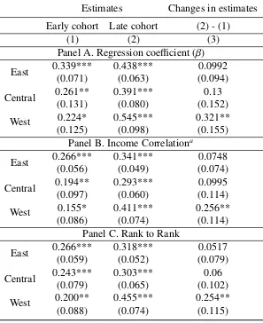
2.3 Intergenerational Income Mobility by Region . . . 103

2.4 Absolute vs. Relative Intergenerational Income Mobility in East, Central, and West China . . . 104

2.5 Intergenerational Education Mobility . . . 105

2.6 Intergenerational Education Mobility byHukouStatus . . . 106

2.7 Intergenerational Education Mobility by Region . . . 107

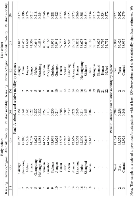
2.8 Absolute vs. Relative Intergenerational Education Mobility in 22 Provinces or Municipalities . . . 108

2A.1 Summary Statistics on the Chinese Household Income Projects Data . . . 120

2A.2 Quintile Transition Matrix of Intergenerational Income Mobility . . . 121

2A.3 Summary Statistics on the Chinese Family Panel Studies Data . . . 122

2A.4 Quintile Transition Matrix of Intergenerational Education Mobility . . . . 123

3.1 Summary Statistics . . . 146

3.2 Estimates for Intergenerational Income Elasticity and Intergenerational Income Correlation in China’s Transition Period . . . 147

3.3 Relationship between Mediating Variables, Child’s Income, and Parental Income in China’s Transition Period . . . 148

(9)

3.5 Relationship between Mediating Variables, Child’s Income, and Parental Income by Income Group in China’s Transition Period . . . 150 3.6 Account for the Contribution of Educational Attainment, Party

Member-ship and OwnerMember-ship of Work Unit to Intergenerational Income Elasticity by Income Group in China’s Transition Period (Percentage) . . . 151 3.7 Relationship between Mediating Variables, Child’s Income, and Parental

Income by Income Group in China’s Transition Period: Robustness Test . 152 3.8 Account for the Contribution of Educational Attainment, Party

Member-ship and OwnerMember-ship of Work Unit to Intergenerational Income Elasticity by Income Group in China’s Transition Period: Robustness Test (Percent-age) . . . 153

(10)

List of Figures

1.1 Illustration of Rustication Dynamics in an Optimisation Problem with

Multiple Steady States . . . 41

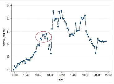
1.2 Number of Births in China (1930 - 2010) . . . 41

1.3 Number of Rusticated Youths . . . 42

1.4 Rustication Rate in Each Cohort . . . 42

1.5 Migration in the Rustication . . . 43

1.6 Variation in the Possibility of Rustication by Father’s Educational Status . 43 1.7 An Illustration on the Spill-over Effect of Rustication . . . 44

1.8 Data Coverage in the Chinese Household Income Project 2002, Chinese Twins Survey 2002, and mini-census 2005 . . . 44

1.9 Rustication Rate and City Population in 1953 . . . 45

1.10 Senior High School Rate in Each Cohort . . . 45

1.11 Average Logarithm of Monthly Income in Each Cohort . . . 46

1.12 Housing Size (square metres) in Each Cohort . . . 46

1A.1 Variation in the Possibility of Rustication by Father’s Social Status . . . . 56

2.1 Per Capita GDP and Gini Coefficient in China . . . 92

2.2 International Comparison of Gini Coefficients . . . 92

2.3 Government Educational Expenditure/GDP . . . 93

2.4 Return to Education in Urban China . . . 93

2.5 Increase in Tuition in China . . . 94

2.6 Return to Schooling Years by Gender . . . 94

2.7 Central and Local Governmental Expenditure on Education . . . 95

2.8 Annual Wage of Urban Workers . . . 95

2.9 Primary School Enrolment Rates and Secondary School Progression Rates 96 2.10 Tertiary School Enrolment Rates . . . 96

2.11 Schooling Years by Gender and by Region . . . 97

2.12 Return to Schooling Years by Province . . . 97

2.13 Logarithm of the Income of Children vs. Logarithm of the Income of Parents . . . 98

2.14 Income Rank of Children vs. Income Rank of Parents . . . 98

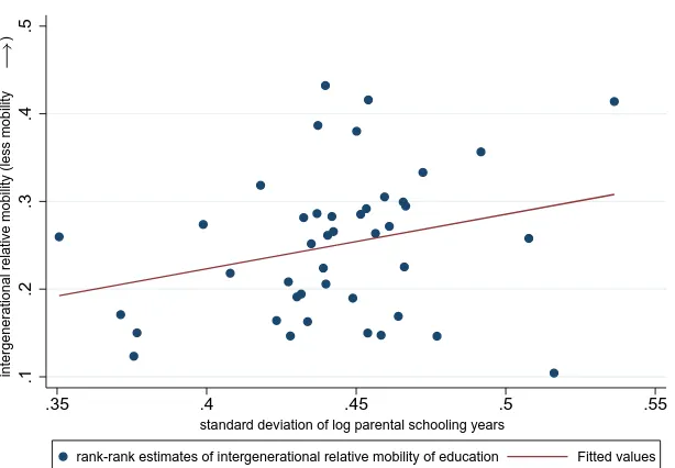
2.15 Income Rank of Children vs. Rank of Parents in Early and Late Cohorts . 99 2.16 Schooling Rank of Children vs. Rank of Parents in Early and Late Cohorts 99 2.17 Relative Mobility vs. Standard Deviation of Parental Schooling . . . 100

2.18 Absolute Mobility vs. Standard Deviation of Parental Schooling . . . 100

(11)

2A.2 Absolute Intergenerational Income Mobility in Early Cohort . . . 115

2A.3 Relative Intergenerational Income Mobility in Late Cohort . . . 116

2A.4 Absolute Intergenerational Income Mobility in Late Cohort . . . 116

2A.5 Relative Intergenerational Education Mobility in Early Cohort . . . 117

2A.6 Absolute Intergenerational Education Mobility in Early Cohort . . . 117

2A.7 Relative Intergenerational Education Mobility in Late Cohort . . . 118

2A.8 Absolute Intergenerational Education Mobility in Late Cohort . . . 118

2A.9 Relative Mobility vs. Gini Coefficient of Family Income . . . 119

2A.10Absolute Mobility vs. Gini Coefficient of Family Income . . . 119

3.1 Provinces and Municipalities under the Chinese Household Income Project (CHIP) . . . 145

(12)

Preface

Inequality is a rising concern in developing countries. In this thesis, I examine intragener-ational and intergenerintragener-ational inequality in the largest developing country, China. Specif-ically, the thesis analyses the long-term consequences of the largest forced migration in history, estimates intergenerational mobility in education and income in the contemporary era, discusses the mechanism of intergenerational income transmission, and examines the interaction of cross-sectional inequality and intergenerational mobility.

The thesis contains three essays. The first investigates the long-term consequences of early adversity on economic behaviours, using the largest forced migration experiment in history. From 1966 to 1978, 17 million urban youths in China, mostly junior or se-nior high school graduates, were sent under a rustication policy to the countryside to do farm work for an average of three to four years. Using difference-in-difference estimation with data from the 2005 mini-census, I find that the rusticated generation behaves more conservatively than their earlier and later counterparts. They spend less on housing and purchase more insurance and pension. The intragenerational estimates reveal the same conservative pattern as the intergenerational research. Compared to their age-eligible but non-rusticated peers, the rusticated individuals spend less on housing, accumulate more savings and insurance, and invest less in risky assets. Based on data from the Chinese Household Income Project and Chinese Twins Survey in 2002, the results remain robust under both Ordinary Least Squares (OLS) and twin fixed-effects estimations. I demon-strate that one interpretation of the conservative behaviour lies in the habits shaped during adversity.

(13)

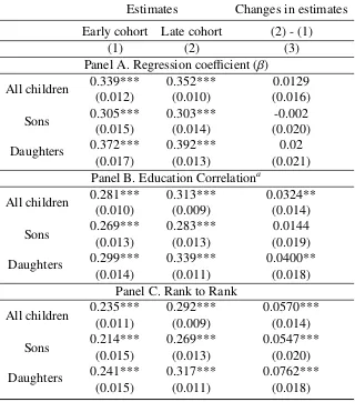
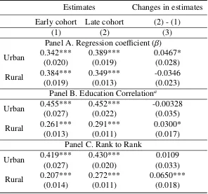
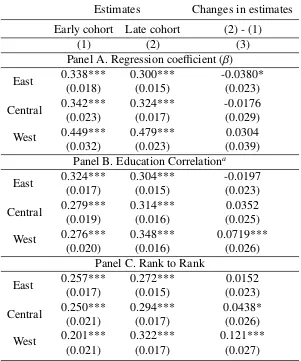
In addition to the intragenerational inequality, I investigate in the second chapter in-tergenerational mobility in China’s present transitional period, as well as its interplay with cross-sectional inequality. This chapter is written jointly with Junjian Yi and Junsen Zhang. Our results show that intergenerational mobility in both income and education de-clines sharply along with China’s market reform. This trend is particularly significant for females and residents of economically disadvantaged regions, such as rural and western parts. To interpret these patterns, we develop a conceptual framework from the human-capital perspective (Becker & Tomes, 1979, 1986; Solon, 2004; Corak, 2013). We explain the changes in China’s intergenerational mobility with reference to five factors: return to human capital, cost of education, government policies on human-capital investment, household income, and income inequality. Linking cross-sectional inequality to intergen-erational mobility, we draw a Great Gatsby Curve with a negative slope to understand the dynamic interplay of the two. Intergenerational mobility has declined with the increase in cross-sectional inequality since China’s economic reform. Poor families benefit less from this growth than rich families do. Given this decline, China’s cross-sectional inequality is expected to increase in the future.

To the best of our knowledge, this is the first study to systematically explore the dy-namic interplay of inequality and mobility in China. It contributes to the literature on intergenerational mobility (Black & Devereux, 2011; Chettyet al., 2014a,b), and stands out as the first analysis of its patterns with respect to cohort, gender, and region in China’s reform era. Moreover, we present the first attempt to relate declining intergenerational mobility to the rising cross-sectional inequality in China by finding a negatively sloped Great Gatsby Curve. It may enrich understanding of the dynamic evolution of inequality in other transitional or developing economies.

In the third chapter, I investigate the channels for intergenerational income transmis-sion during China’s economic transition. In addition to the conventional channel of edu-cation, I examine two new ones, political and occupational identities. Using the decom-position method (Bowles & Gintis, 2002; Blandenet al., 2007), I discover that for both rich and poor families in the pre-reform era, the conventional channel of education acts as the leading contributor to intergenerational income persistence. In the post-reform era, however, the leading contributor varies across income groups. Education still contributes most to the income persistence across generations in poor households. For the rich, it is the political identity of Communist Party member that leads. The effect of occupational identity as working in the state-owned sector is less important in both types of household in the post-reform period than that in the pre-reform era.

Different from the literature which focuses on the transmission of educational

(14)

(15)

Chapter 1

Does Adversity A

ff

ect Long-Term Consumption and

Fi-nancial Behaviour? Evidence from China’s Rustication

Programme

1

Does adversity affect long-term economic behaviour? How does a policy influence one generation over the long term? In the first chapter, I examine the long-term conse-quences of adversity on consumption and financial behaviour, using the largest forced migration experiment in history.

From 1966 to 1978, 17 million urban youths in China, mostly junior or senior high school graduates, were sent to the countryside to do farm work for an average of three to four years under a rustication policy. Using data from the mini-census in 2005, I find that the rusticated generation behaves more conservatively than the non-rusticated gener-ations over the long term, as they consume less housing and purchase more insurance and pension.

In addition to the cross-generational influence, I investigate the intra-generational ef-fects of rustication with data from the Chinese Household Income Project in 2002 and the Chinese Twins Survey in the same year. A similar conservative behavioural pattern is revealed. Individuals with rustication experience spend less on housing, accumulate more savings and insurance, and invest less in risky assets, compared to their age-eligible but non-rusticated peers. Applying a habit-forming model, I suggest that one interpretation for the conservative behaviour lies in the habits formed during adversity. The results shed light on how a policy, especially in the early stage of life, influences one generation over the long term.

As the first chapter of the thesis, it starts with an investigation of inequality with a focus on the historically under-represented group - the rusticated population. This chap-ter examines how early experience affects one generation, and lays foundation for the analyses of intergenerational inequality and its interplay with cross-sectional inequality in chapters 2 and 3.

1_{A preliminary version of this chapter began circulating in 2013 with the title “Adolescent Shock,}

Resilience, and Long-Run Effects on Income and Consumption”.

(16)

1.1

Introduction

Does adversity affect long-term consumption and financial behaviour? How does a policy influence one generation over the long term? I aim to address these two questions in this paper. Literature in economics, sociology, and psychology demonstrates evidence to sup-port the correlation between early life experience and later economic behaviour. In the literature for the Great Depression, Malmendier & Nagel (2011) find that macroeconomic experiences influence individuals’ risk taking behaviour. The generation which experi-enced the Great Depression tends to take fewer financial risks throughout their lives. They also have a markedly lower consumption of durable goods, as shown in Romer (1990) and Crafts & Fearon (2010). Schoar & Zuo (2013) examine the managerial styles of CEOs, and find that those entering the labour market during recession periods behave in a more conservative way.

Similar evidence is revealed among studies on the median- or long- term effects of military service or wars. Benmelech & Frydman (2014) study the behaviour of CEOs with military experience, and find that they are associated with conservative corporate policies and ethical behaviour. Blattman (2009) and Bellows & Miguel (2009) indicate that war violence changes individuals’ political attitudes. They are more likely to join local political groups and vote after wars. With respect to other life adversities, Alesina & La Ferrara (2002) and Castillo & Carter (2007) present empirical evidence that people with traumatic experiences, such as disease or divorce, have less trust in others but show more altruism.

(17)

echo the literature (Deng & Treiman, 1997; Xieet al., 2008; Yang & Li, 2011).

I apply difference-in-difference, ordinary least squares (OLS), and fixed-effects esti-mations to the mini-census in 2005, the Chinese Household Income Project in 2002, and the Chinese Twins Survey in 2002 respectively, to examine the cross- and intragener-ational impacts of rustication. To start with, I apply difference-in-difference strategy to the mini-census in 2005 to depict the general behavioural pattern of the rusticated versus non-rusticated generations. Rustication varies across cohort and region. The generation of 1946-1961 were subject to the policy, with almost half of the population rusticated in practice. Cohorts born before 1946 or after 1961 were rarely sent to the countryside. In addition, rustication was more severe in large cities than small ones as the revolutionary propaganda was much stronger and coercion was enforced (Deng & Treiman, 1997). I find that the rusticated generation behaves more conservatively in consumption and fi-nance than the non-rusticated cohorts. They live in smaller houses, spend less on housing purchase, and buy more insurance and pension even after three to four decades. These findings are consistent with the literature that individuals experiencing economic reces-sion tend to spend less on durable goods (Romer, 1990; Crafts & Fearon, 2010), and have a lower willingness to take financial risk (Malmendier & Nagel, 2011; Schoar & Zuo, 2013; Benmelech & Frydman, 2014).

Rustication was announced as compulsory for all age-eligible high-school graduates at the start. However, the quotas of rustication varied according to economic situation and policy changes. When the quota was less than 100% (not all high-school graduates were required to be rusticated), some selection occurred (Liet al., 2010). There are two types of selection in the rustication. First, there exists cross-household selection, as the previously privileged families (such as the rich and/or educated) lost power in the social re-shuffle and were less able to help their children acquire exemptions from rustication (Zhou & Hou, 1999; Liet al., 2010). Second, there is within-household selection. In the case of a binding quota, the parents had to choose which child(ren) to be rusticated. To overcome the potential endogeneity, I specify two empirical strategies. On the one hand, I explicitly control fathers’ socioeconomic traits as proxies for the family background in the OLS estimation, with data from the 2002 Chinese Household Income Project in absence of the co-residency bias.2 _{On the other hand, I apply twin and sibling fixed-e}ff_{ects estimations}

to the 2002 Chinese Twins Survey, which is the first dataset on twins in China. Bias from common family background is eliminated. In addition, the within-household selection is largely reduced in the specification for identical twins, as they are genetically the same,

2_{The 2002 Chinese Household Income Project collects socioeconomic information on parents, despite}

their living separately or being deceased. Thus it overcomes the co-residency bias in conventional household surveys.

(18)

and have far less difference than non-identical twins or siblings that are further apart (Li

et al., 2010). Moreover, I specify a robustness check controlling the difference between

identical twins using birth weight as a proxy for initial endowment following the literature (Rosenzweig & Wolpin, 1995; Behrman & Rosenzweig, 2004).

Just as with the difference-in-difference estimation, I find that individuals with rus-tication experience behave more conservatively than their age-eligible but non-rusticated peers. They spend less on housing consumption, save more, purchase more insurance, and invest less in risky assets such as stocks and bonds. Consistently across the three empirical strategies, I find that rustication decreases lifetime schooling, but does not have a signif-icant influence on long-term income, as shown in previous studies (Meng & Gregory, 2002, 2007; Xieet al., 2008; Yang & Li, 2011). The results remain robust if the potential influence from initial endowment, occupational choice, and spousal traits is taken into account.

Why do the rusticated individuals behave conservatively? With a simple habit-forming model, I consider one interpretation lies in the habits shaped during adversity (Becker & Murphy, 1988; Orphanides & Zervos, 1994; Crawford, 2010; Costa, 2013). Take hous-ing for instance: given that the past and current consumption of habit-formhous-ing goods are complementary, the habit of depressed housing consumption formed during the rustica-tion leads the later consumprustica-tion to converge to a low steady state.3 Empirical evidence examining the influence from the incidence versus the intensity of rustication supports the habit explanation. I find that it is mainly the rusticated years (the intensity) rather than the participation in the programme itself (the incidence) that contributes to the findings. The longer the rusticated period, the more likely is the convergence to a steady state of housing consumption. Interview evidence also supports this interpretation. The sent-down youths self-reported that they learned about the toughness of life from the adverse experience in rural areas (Zhou, 2013). It is consistent as well with the evidence on the role of habits and values as determinants for behaviour and socioeconomic changes, such as the rise of the middle class during the Industrial Revolution and modern capitalism (Doepke & Zili-botti, 2008; Weber, 2013). What is worth mentioning is that the habit explanation does not exclude other possible interpretations. Various channels could co-exist, interact with each other, and influence long-term economic behaviour together.

Forced migration to rural areas happened in countries other than China, though none is comparable to its huge population and age concentration in adolescence. Indonesia had a Transmigration programme through the 20th_{century, moving landless people from}

3_{During the rustication, the sent-down youths lived in small shabby houses, called}_{“collective units”}

(19)

densely populated areas to less populous areas. The total population influenced was around five million (Fearnside, 1997). The Soviet campaign, Dekulakization, deported better-offpeasants and their families to distant parts of the Soviet Union and other parts of the provinces between 1929 and 1932. More than 1.8 million rich peasants were de-ported during the peak time of 1930-1931 (Conquest, 1987; Viola, 2007). Russia’s Virgin Lands Campaign between 1954 and 1963 was considered the predecessor for China’s rus-tication programme. Advertised as a socialist adventure, 300,000 youths travelled to the Virgin Lands in the summer of 1954 (Taubman, 2004). Another parallel can be drawn with the U.S.’s Indian Removal in the 19th century. About 70 thousand Indians were forcibly relocated to designated territories, because of population density concerns and the availability of arable land. Nonetheless, China’s rustication programme affects a huge population of 17 million, and has a demographic concentration on adolescence when the attitude towards the world is first established (Ghitza & Gelman, 2014).

To the best of my knowledge, this is the first paper that systematically investigates the long-term impacts of this biggest inner-country migration on economic behaviour. Pre-vious studies focused on its impacts on education and income (Meng & Gregory, 2002, 2007; Xieet al., 2008; Yang & Li, 2011). Other literature touches upon its influence on mentality or consumption, though with little empirical evidence or focusing on the out-come of household appliances (Zhanget al., 2007; Zhou, 2013). Given that rustication shifts urban youths’ privileged status into an unprivileged rural one during their adoles-cence when values are established, its impacts on behaviour are expected to be profound and worthy of investigation. In this study, I try to provide empirical evidence and expla-nation to locate the heterogeneity in economic behaviour. The study also sheds light on how a policy, pertaining to those in the early stage of life, exerts long-term impacts on a generation through changing their behaviour. The policy implication lies in the impor-tance of later policy interventions if the policy makers take the long-term influence of one policy on economic behaviour into account.

The remainder of the paper is organised as follows. Section 1.2 specifies the theo-retical framework. Section 1.3 provides institutional background on China’s rustication programme. Section 1.4 describes three data sets followed by Section 1.5 which speci-fies corresponding empirical specifications. Section 1.6 presents and discusses empirical results. Section 1.7 draws conclusion.

(20)

1.2

Theoretical Framework

1.2.1 Set-Up

I adopt a habit-forming model to elaborate the long-term effects of rustication (Becker & Murphy, 1988; Abel, 1990; Orphanides & Zervos, 1994, 1995; Crawford, 2010). Suppose an individual has two consumption goods at period t: an ordinary good ct with price

1, and a habit-forming good ht (eg., housing consumption) with price p. Her current

utility, u(ct,ht,st), depends on ct, ht, and a measure of stock of past consumption st,

which depends onhtbut notct. The individual accumulates her future stock from previous

consumptionstandht. The evolution of stock is described below:

st+1 =δst +ht,

whereδ is the depreciation rate of the past consumption stock. Through st and ht, st+1

enters the current utilityu(ct,ht,st). Her incomey, is set constant following the literature

(Becker & Murphy, 1988; Orphanides & Zervos, 1994, 1995). The maximisation problem is:

V(s0)= max

∞

X

t=0

βt

u(ct,ht,st) (1)

s.t. ct+ pht ≤y, (2)

st+1 =δst+ht. (3)

Following Orphanides & Zervos (1994), the utility functionu(ct,ht,st) follows the

com-plementarity assumption that the current consumptionht and the past consumption st are

complements (uhs > 0). In addition, this complementarity is stronger than that betweenc

ands(uhs ≥ucs).4

Along an optimal path, the budget constraint (2) binds. By substitutingct =y−phtinto

the utility function, the objective function can be redefined asx(ht,st)≡u(y− pht,ht,st),

which is a function ofht andst only. Rewrite the maximization problem (1) in a dynamic

programming framework:

V(s)=max

h [x(h,s)+βV(δs+h)]. (4)

The correspondence describing the optimal consumption path is: φ∗(s) ≡ {s0|V(s) =

x(s0 −δs,s)+ βV(s0)}. ¯s is a steady state if ¯s ∈ φ∗( ¯s). Define sc as a critical level if

4_{The other three assumptions of the utility function are: Assumption 1. the function}_u₍_c_,_h_,_s_{) is}

second-order continuous forc,h,s≥0. Assumption 2. the functionuis increasing and strongly concave incand

(21)

the optimal local dynamic diverges around it. Following Proposition 1 in Orphanides & Zervos (1994), the optimal paths are described as below:

Proposition: The optimal paths converge to a steady state monotonically from any initial

stock; if the initial stock lies between two consecutive steady states, the optimal paths converge to either one or the other; exactly one critical level exists between any two con-secutive stable steady states (Orphanides & Zervos, 1994).

1.2.2 Modelling the Impact of Rustication

I take the long-term impact of rustication on housing consumption as one instance to illustrate the incorporation of rustication into this model. Housing is habit-adjusted as discussed in the literature (Huang, 2012). Denote s0 the initial individual stock of

con-sumption at the start of rustication, and τ the duration of rustication. Define h∗(s) the optimal unconstrained housing consumption, where s is the stock of past consumption. During the rustication, the housing consumption is depressed, as the sent-down youths lived in small shabby houses called“collective units”, which were shared with many oth-ers.5 _{Thus I impose a cap on the housing consumption during the rustication, consistent}

with previous research (Costa, 2013). Set:

ht =h¯ < h∗(s0),∀t∈[0, τ]. (5)

From the budget constraint (2),ct = c¯ = y− ph¯,∀t ∈ [0, τ]. Inserting ¯hinto eq.(3) and

iterating, I obtain the stock of consumption at the end of rustication:

sτ(s0)= δτs0+

1−δτ

1−δh¯, s0 given. (6)

If at the end of the rustication, the stock of consumption sτ(s0) is less than the critical

level sc_{, the housing consumption} _h

t will converge to a low steady state. Figure 1.1

illustrates the dynamics, with housing consumption on the vertical axis and the stock of consumption on the horizontal axis. The graphing follows Orphanides & Zervos (1995) and Costa (2013). Assume an individual is at the steady state s0 = sh initially. During

the rustication, she is forced to consume below ¯h, reducing her stock of consumption over the rustication period,τ. If by the end of the rustication, the stock of consumption sτ(s0)

is less than a critical point sc (sc < s0), she will enter a new optimal path converging

to a new stable steady state with lower housing consumption. Alternatively, if the stock

5_{Even by the end of 1976, about 1 million rusticated youth still did not lived in proper dwellings,}

especially for those married couples (Bonnin, 2013).

(22)

of consumption after the rustication does not drop below any critical value, the housing consumption will converge back to the original level. To summarise:

Prediction: After the rustication, if an individual’s stock of housing consumption

drops below a critical level, she will enter a new optimal path converging to a steady state with lower utilization of housing consumption.

From the conventional budget constraint with saving, an increase in the financial assets is expected from the decreasing consumption as demonstrated in the prediction above.

What is worth mentioning is that the habit channel could co-exist with other channels, such as the changing risk aversion or discount rate.6 However, those mechanisms are not mutually exclusive. Moreover, they interact with each other, and shape the long-term economic behaviour together.7

1.3

Institutional Background

From 1966 to 1978 during China’s Cultural Revolution, approximately 17 million urban youths (1/10 of the urban population), most of whom were junior or senior high school graduates, were sent to the countryside (Liet al., 2010). With no access to formal educa-tion, they spent 3-4 years on average in the rural area. They did heavy manual farm work for 12 hours per day and 7 days per week, as documented in Bernsteinet al. (1977) and Zhou (2013). More than 90% returned to the cities by 1980, two years after the official end of the Cultural Revolution (Bonnin, 2013). About 5% never returned having married local peasants or found employment in non-agricultural jobs in rural areas (Zhou & Hou, 1999).

1.3.1 Origins and Rules of the Rustication

The earliest documented rustication was in 1955. It was small scale with less than 8,000 individuals affected (Bonnin, 2013). Large-scale rustication was initiated in 1966, with the start of the Cultural Revolution. In the first two years of the Cultural Revolution, primary schools, high schools, and universities were shut down. Many urban youths participated in the revolutionary activities. The rustication was made official in 1968,

6_{For instance, when the rusticated youths returned to cities, they were subject to fewer resources}

com-pared to their non-rusticated peers because of the lost years in the countryside. Poor economic status is associated with high risk aversion (Binswanger, 1981; Guiso & Paiella, 2008). To prepare for future rainy days, the rusticated youngsters are expected to consume less, save and insure more, and invest less in the risky assets. In addition, it is also plausible that the discount rate alters among the rusticated youths. They discount the future less and save more.

7_{For instance, the wealth e}_ff_{ect after returning to cities could interact with the habit-forming channel,}

(23)

as Mao urged the urban youths to go to the rural areas to be re-educated by the farmers (Zhanget al., 2007; Liet al., 2010). Most were unwilling to be separated from families, and thus coercive techniques such as threatening parents with job loss were used (Deng & Treiman, 1997).

In addition to the revolutionary propaganda, rustication was motivated by deep eco-nomic concerns. The rising urban unemployment was an important cause for the large-scale rustication. Interrupted by the Cultural Revolution, senior high schools and uni-versities closed and did not admit new students until 1971/1972. When they reopened, senior high schools did not recruit old students who missed the chance in previous years (Meng & Gregory, 2002). Universities did not admit senior high school graduates di-rectly (Liet al., 2010). The recruiting criterion was not academic merit, but performance in the Cultural Revolution (e.g.,participation in the rustication), political attitude, or fam-ily background.8 _{The dysfunction of senior high schools and universities in absorbing}

graduates served to increase youth unemployment. In addition, shortly after the founda-tion of the People’s Republic of China in 1949, the baby boom enhanced the employment pressure among urban youths (Banerjeeet al., 2010; Zhou, 2013). The red line in Figure 1.2 circles the first baby boom shortly after 1949. Those children were of high-school age when the Cultural Revolution started, and would enter the labour market if there was no rustication.

The local government had yearly send-down quotas to meet. The quota varied ac-cording to the economic situation and policy changes. Figure 1.3 depicts the number of rusticated youths migrating into rural areas (Kojima, 1996). From 1967 to 1968, approxi-mately 2 million people were sent to the rural areas. This number peaked at 2.67 million in 1969 (Kojima, 1996; Bonnin, 2013). With the economic recovery and increasing supply of urban jobs, the number of rusticated youths dropped in the following years. A second peak appeared around 1975 when the four leaders of the Revolution, called the“Gang of

Four”, seized power and strongly advocated rustication using patriotic propaganda (Bai,

2014).

1.3.2 Variation Across Cohort and Region

The majority of the rusticated youths were junior or senior high school graduates. I focus on the cohorts born between 1946 and 1961 following the literature (Li et al., 2010). The earliest birth cohort of 1946 contains the senior high school graduates in 1966 when

8_{Section 1.3.3 discusses the role of family background on rustication in detail.}

(24)

large-scale rustication began.9 The latest birth cohort of 1961 includes the junior high school graduates in 1978 when the rustication programme was officially ended. Figure 1.4 graphs the rustication rate in each cohort. It validates the specification on the treated generation between 1946 and 1961. For cohorts out of this range, the rustication rate is less than 10%.

The destination of rustication also varies, depending on the home cities and time of rustication. Bonnin (2013) documents that most rustication was within the province and students were sent to the nearby countryside. However, there was about 8% cross-province migration, mostly from big municipalities to the remote frontiers. Figure 1.5 demonstrates the direction of cross-province migration. It was concentrated in the three biggest municipalities (Beijing, Tianjin, and Shanghai), but also included other provincial capitals such as Wuhan and Chengdu. The destinations were the remote frontiers, such as Heilongjiang in the northeast, Xinjiang in the northwest, and Yunnan in the southwest. Because of the variation of rustication across cohort and region, I adopt a diff erence-in-difference estimation to capture the generation effect of rustication. Details are displayed in Section 1.5.1.

1.3.3 Potential Endogeneity

Rustication was announced as compulsory for almost all age-eligible high school grad-uates at the beginning. Nevertheless, when the sent-down quota was binding (not all high school graduates were requested to be rusticated), some selection occurred. There was cross- and within- household selection during the rustication (Zhou & Hou, 1999;

Li et al., 2010). On the one hand, the possibility of being sent to the countryside

var-ied across households. This is because the previously privileged families (eg., the rich and/or the educated) lost power in the social re-shuffling of the Cultural Revolution. Thus they are less able to help their children acquire exemptions from rustication. One the other hand, children from previously unprivileged families with parents who were work-ers, farmwork-ers, or soldiers during that time period, were more likely to be able to inherit their parents’ jobs or join the army. Thus they were able to return to cities earlier, or even be exempted from rustication. In the 1970s, the rustication policy was relaxed. A small proportion of junior high school graduates, most with favoured family backgrounds, were directly admitted into senior high schools.

Figure 1.6 displays one instance of how the possibility of rustication varies with family

9_{During that period, children were admitted into primary school around the age of 8. Primary-school}

(25)

background. The bar indicates the possibility of being rusticated. Numbers in brackets indicate observations in each category with percentages in the parentheses. A majority of the fathers have educational level at elementary school level (35.6%), followed by those who with no schooling (29.3%), with junior high school level (18.3%), and with senior high school level or above (16.8%). Clearly, children from previously privileged family backgrounds, such as those with fathers who were intellectuals, had a higher probability of being sent to the countryside. This is because intellectuals were considered elites before the Cultural Revolution, and were against in the programme. A similar scenario applies to children of enterprise owners, as shown in Figure 1A.1. However, the magnitude of selection is small, with less than 5% conditional on fathers’ educational level, or less than 10% on their social status.

In contrast, there is within-household selection in addition to the cross-household se-lection (Liet al., 2010). Parents had to choose the child(ren) to go to the countryside if not all children were requested for rustication. Different empirical strategies are applied to address the cross- and within- household endogeneity, and will be described in Section 1.5.

1.4

Data

I use three data sets, each of which is associated with one empirical specification, to exam-ine the long-term effects of rustication on housing consumption and financial behaviour. The three data sets supplement each other and are described as below.

1.4.1 Mini-Census 2005

I first use the 2005 mini-census to describe the behaviour of the rusticated generation versus non-rusticated generations. The generation experiencing rustication is expected to behave in a different way from their earlier or later counterparts, as almost half of them were rusticated, and the effect could spill over to other age-eligible but non-rusticated individuals. Figure 1.7 illustrates examples of the spill-over effects. For instance, the surge of population returning to cities after the programme may generate a demand shock on urban housing.10 Importantly, the cross-generation investigation is not subject to the cross- or within- household selection as described in Section 1.3.3.

The mini-census was implemented from November 1 to November 10 in 2005 by the National Bureau of Statistics of China and the office of the 1% population sampling

10_{The rustication programme was ended o}_ffi_{cially in 1978. In the following year, 3.95 million rusticated}

youths returned to cities (Kojima, 1996).

(26)

investigation in the State Council of the People’s Republic of China. It covered 1% of the national population, or approximately 13,000,000 observations. The data I use covers 20% of the mini-census. My sample focuses on the urban areas, since the target of the large-scale rustication policy was urban educated youths. Rural residents and urban-to-rural migrants are excluded.11

The merits of using this data set are two-fold: first, the sample covers all provinces and is representative of the general population. My sample contains approximately 1 million observations with intact information on education and income. The sampling is according to the population in each province, autonomous region, and municipality, and thus representative of the general population. Second, unlike the population census, the mini-census asks detailed questions on housing size, purchasing price, insurance, and working time, in addition to education and income. It provides a rare opportunity to investigate the overall pattern of consumption and financial behaviour across China.

The summary statistics are presented in Column (1) of Table 1.1. Individuals are in their late 40s in 2005 and are sex balanced (52% are male). Almost half (45%) of the sample has at least a senior high school level of education in 2005, but only 5% achieves university level. The annual income is 1,630 U.S. dollars (USD) in 2002 values. The average housing size is 59 square metres, with an estimated market housing price of 7,645 USD in 2002 values. The average working hours are 46 hours per week, or approximately 9 hours per day.12 Concerning insurance purchase, 30% of the population have unemployment insurance. The proportion of pension and health insurance almost doubles, possibly because of the average age being in the late 40s, when old-age support and medical care become increasingly important.

One possible caveat lies in no direct measurement on rustication being available in the mini-census. However, as I am interested in the cross-generational influence, this information is not necessarily needed. The following two datasets provide detailed rus-tication information at the individual level, which examines the intra-generational effects of rustication.

1.4.2 Chinese Household Income Project 2002

I apply the 2002 Chinese Household Income Project (CHIP 2002) to examine the intra-generational effect of rustication. CHIP 2002 is a joint research study sponsored by the In-stitute of Economics at the Chinese Academy of Sciences, the Asian Development Bank,

11_{Migrants from rural to urban areas still hold rural registration (}_Hukou_{), and do not have equal access}

to the same educational and occupational opportunities as urban citizens.

(27)

the Ford Foundation, and the East Asian Institute at Columbia University. Consistent with the previous strategy, I focus on urban residents only. The data covers 54 cities or municipalities from 11 provinces in China, as marked in dark grey in Figure 1.8.

The advantages of using CHIP 2002 data to analyse the long-term impacts of rustica-tion lie in the following features. First, the CHIP project provides rich data on rusticarustica-tion and outcome variables. The survey asks each individual above 35 years old about the ex-perience of rustication and the length of time one was sent to the countryside. In addition, it records the individual’s housing consumption (housing size and market price), saving, investment portfolio, expenditure on insurance, as well as working time, occupation, ed-ucation and income. It provides a rare opportunity to investigate the consequences of rustication from various perspectives. Secondly, it collects information on family back-ground in the absence of co-residency bias. The survey reports socioeconomic status on the parents of household heads and spouses, regardless of whether they live together or are alive. The information contains parental educational levels, social status classified before the Cultural Revolution, and political party affiliation. To the best of my knowledge, this is the only household survey in China that provides such detailed information on family background and overcomes co-residency bias. Last but not least, the area under this sur-vey is geographically and economically representative, which provides an opportunity to yield nationally representative estimates.13

Column (2) in Table 1.1 presents the summary statistics. They are generally the same as those found in the mini-census, with no statistically significant differences reported. Among those age-eligible youths born between 1946 and 1961, 42% have been rusticated. Conditional on being rusticated, the average length of being sent to the countryside is 3.89 years (detailed tabulation of the rusticated years is shown in Table 1A.1). By the end of 2002, they have saved 4,342 USD, which is about three years’ income.14 In addition, they have invested 828 USD in stocks and bonds by the end of that year, which is almost half of their annual income. They also spend 195 USD on insurance, which is about 1/10 of annual income.

13_{CHIP is considered geographically representative as the areas under survey cover the northeast}

(Liaon-ing), the south (Guangdong), the southwest (Yunnan), and the west (Gansu). It is considered to be economi-cally representative as the surveyed areas include the richest parts in China such as Beijing and Guangdong, as well as the least developed parts such as Gansu.

14_{Saving is defined as the summation of fixed and current deposits, stocks and bonds, and others. Other}

sources contain money lent, self-owned funds for family business, investment in enterprises/business (ex-cept stocks and bonds), and monetary value of commercial insurance as a deposit.

(28)

1.4.3 Chinese Twins Survey 2002

The third data set I apply is that of the Chinese Twins Survey in 2002, which is the first twins data set in China, designed by Professors Mark Rosenzweig and Junsen Zhang.15

The survey was carried out by the National Bureau of Statistics in 2002 in five cities in China, depicted in yellow triangles in Figure 1.8.16 _{It includes 1,838 identical twins,}

1,152 non-identical twins, and 1,672 singletons (as control group) aged between 18 and 65. The survey collects information on each twin’s housing consumption, working time, schooling, income, emotional control, and other demographic details, such as age, gender, and number of household members. Similar questions are also asked to their non-twin siblings and singletons in the control group.

My sample contains 602 identical twins and 4,866 siblings born between 1946 and 1961 with intact information on rustication, education, and income.17 _{In addition to}

pro-viding a rich set of outcome variables, I consider the following advantages of using the Twins Survey for this study. First, it contains detailed information on rustication, such as whether individuals were rusticated and for how many years. Second, it facilitates the elimination of bias from cross- and within- household selection, as discussed in Sec-tion 1.3.3. This is because identical twins share similar genetics and have same family background. By adopting a twin fixed-effects strategy, I can eliminate influence from the unobserved family background. In addition, the differences between identical twins are much less than those between the non-identical twins and among further apart siblings. Thus the within-household bias on rustication is much reduced under this strategy. Sim-ilarly, siblings share the same family background although with various genetic traits. The sibling fixed-effects estimation supplements the results from the twin fixed-effects strategy.

Summary statistics on identical twins and siblings are displayed in Columns (3) and (4) of Table 1.1, respectively. They are roughly the same as those presented in the pre-vious two data sets. No statistically significant differences are found for the variables. Specifically, for identical twins born between 1946 and 1961, more than half (54.2%) were rusticated. Almost 30% (180 twins from 90 pairs) of them have within-twin diff er-ence in rustication, which generates the variation in the twin fixed-effects estimation. The variation of rustication within identical twins is demonstrated in Table 1A.2.

15_{Professor Mark Rosenzweig is Frank Altschul professor of Economics at the Yale University.}

Profes-sor Junsen Zhang is Wei Lun ProfesProfes-sor of Economics at the Chinese University of Hong Kong.

(29)

1.5

Empirical Specification

1.5.1 Difference-in-Difference Estimation

Rustication varies across cohort and region, as discussed in Section 1.3.2. Therefore I apply difference-in-difference estimation to the mini-census in 2005 to investigate the generational effect of rustication. The outcome variables contain housing consumption, insurance and pension purchase, as well as working time, education, and income.

The treated generation includes individuals born between 1946 and 1961. The com-parison group contains individuals born between 1940 and 1966 but not in the treated generation. I also specify a complementary strategy as comparing balanced rusticated co-horts of 1946-1950 and 1954-1958versusnon-rusticated cohorts of 1941-1945 and 1962-1966. They are the earliest (1946-1950) and latest (1954-1958) rusticated cohortsversus

the non-rusticated cohorts ahead (1941-1945) and afterwards (1962-1966). Specifically, the 1959-1961 birth cohort is excluded as individuals in that cohort were born during the Great Famine, and may otherwise contaminate the results.

In addition to birth cohort, rustication also varies across region. As documented in Bonnin (2013), the rustication was more severe in big cities, as the revolutionary pro-paganda was stronger and coercion was applied more heavily. To test this argument, I plot the city rustication rate against the logarithm of the city population using the census data in 1953, and present the result in Figure 1.9. A positive and statistically significant coefficient is revealed. With a 1% increase in the city population, the rustication rate is raised by 0.03 percentage points, and is statistically significant at the 5% level. As the average city rustication rate is 0.31 revealed from the Chinese Household Income Project 2002, the 1% rise in the city population indeed increases the city rustication rate by al-most 10%. Consistent with the classification in the City Statistical Yearbook, I define cities with population above 1 million as big cities (NBS, 1985, 2002).18

The empirical specification is as follows:

yict =α1bigc+α2treatedt +α3bigc∗treatedt+Xictαx+µict (7)

wherei stands for individual, c represents city, andt identifies time. bigequals 1 if an individual lives in a big city. Otherwise, it equals 0. The dummy oftreatedequals 1 if an individual was born between 1946 and 1961. It equals 0 if he/she was born between 1940 and 1966 but not in the treated generation. In the complementary specification,treated

18_{The cut-o}_ff_{points of city size are 2 million, 1 million, 0.5 million, and 0.2 million according to the City}

Statistical Yearbook. The range of the population in big cities in 1953 was from 1,091,600 to 6,204,417. The range for small cities was from 26,200 to 916,800.

(30)

equals 1 if an individual was born in 1946-1950 or 1954-1958 cohort. It equals 0 if in either the 1941-1945 or 1962-1966 cohort.

yictis the outcome variable. It includes housing consumption (housing size and price),

pension and insurance purchase (unemployment and health insurance), as well as edu-cation (dummies of having eduedu-cation at senior high school/above or university/above), income (logarithm of income in the last month), and working time (working hours last week). Xict is a vector of control variables, which contain age, ethnicity, gender, and

regional dummies. ict is the disturbance term. Standard errors are clustered at the city

level.

α3 identifies the effect of rustication. One assumption forα3 picking up the influence

of rustication is that there is a parallel trend in outcome variables between big and small cities before the programme. Otherwise, the change may be because of events other than the rustication. Figures 1.10 - 1.12 check those trends. For instance, the senior high school rates in big cities (blue solid line) and small cities (red dashed line) are roughly parallel for cohorts prior to 1946 (Figure 1.10). With the start of the rustication, the senior high school rate remains stagnant in small cities but drops sharply in big cities. The deviation from the preceding parallel trend identifies the effect of rustication. Similar parallel trends are displayed in income (Figure 1.11) and housing consumption (Figure 1.12), which validate my method of difference-in-difference.

A similar specification as that in Eq. (7) is carried out, except the dummy ofbigc is

replaced with a continuous variable of city population in 1953:

yict = β1pop53c+β2treatedt+β3pop53c∗treatedt+Xictβx+ξict (8)

where pop53c is the logarithm of city population in 1953. Others variables remain the

same as in Eq. (7).

1.5.2 OLS Estimation Controlling Family Background Explicitly

With application to the Chinese Household Income Project in 2002 as described in Section 1.4.2, I specify OLS regression controlling family background explicitly as follows:

yi = γ1rusi+γ2f amilyi+Xiγx+i (9)

The sample is restricted to individuals born between 1946 and 1961. Standard errors are clustered at the city level andyiis the outcome variable. It includes housing consumption

(31)

examines individual allocation of net consumption wealth. It also contains education (senior high school/above or university/above), income (logarithm of annual income), and working time (monthly working days and daily working hours).

rusi is the interested independent variable. It is either a dummy for being rusticated,

or the total rusticated years. f amilyi is a vector indicating family background, which

in-cludes dummies for fathers’ social status, educational level, and political status. Xi is a

vector of control variables, including age, ethnicity, gender, and provincial dummies in all specifications. Additional controls vary slightly in different regressions. In the speci-fication for housing consumption, I control education, income, and number of household members. In the specification for financial behaviour, education and income are addi-tional controls. In the specification for income, I follow the literature (Mincer, 1974; Li

et al., 2010) by controlling for schooling, working years, and the squared form. Schooling

is included as one additional control in the equation for working time.

1.5.3 Twin and Sibling Fixed-Effects Estimation

Regressions under twin fixed-effects follow conventional specification in the literature (Li

et al., 2007, 2010). Conditional on the data availability, my empirical work focuses on

estimating the effects of rustication on housing consumption, working time, education and income, with data from the Chinese Twins Survey. The econometric specifications are as below:

y1j = λ1rus1j+ZjλZ+X1jλX +µj+e1j+ε1j (10)

y2j = λ1rus2j+ZjλZ+X2jλX +µj+e2j+ε2j (11)

where the subscript j indicates family. The subscripts 1 and 2 refer to twin orders. All identical twins born between 1946 and 1961 were age-eligible for the rustication. yi j

(i= 1,2) is the outcome variable, which includes housing consumption (housing size and property rights), working time (monthly working days and weekly working hours), edu-cation (dummies for having eduedu-cation at senior high school/above or university/above), and income (logarithm of income in the last month). rusi j (i = 1,2) is the interested

in-dependent variable. Similar to that in the OLS estimation, it indicates a dummy for being rusticated or the total rusticated years.

Zj is a vector of observed family variables, such as regions, which are the same for

identical twins. Xi j (i = 1,2) is a set of twin-specific control variables, which differ

slightly in the regressions for different outcome variables. Specifically, in the specifica-tion for housing consumpspecifica-tion,Xi j contains age, gender, schooling, number of household

(32)

members and logarithm of monthly income. In the specification for working time, Xi j

contains schooling years, in addition to the common controls of age and gender. In the regression for logarithm income,Xi j includes additional controls of schooling years,

ex-perience, and square form of exex-perience, as under the OLS estimation.µjstands for

unob-served family effect, such as parents’ social, educational, or political status. ei j (i = 1,2)

indicates unobserved twin-specific endowment, such as ability, andεi j is the disturbance

term. Standard errors are clustered at the household level.

Estimate ofλ1under OLS estimation is biased because children from previously

priv-ileged families are more likely to be sent to the countryside, as discussed in Section 1.3.3. However, it is difficult to find proxies to identify unobserved family effect µj and

twin-specific endowmentei j, which are possibly correlated withrusi j. To address the bias in

OLS estimates, I apply fixed-effects estimation to identical twins. By taking difference between Eqs. (10) and (11), the fixed-effects estimatorλ1below is obtained:

y1j−y2j =λ1(rus1j−rus2j)+(X1j−X2j)λX+ε1j−ε2j (12)

The unobserved family effectsµjare eliminated as twins share the same family

back-ground. Because identical twins are genetically the same, the influence from twin-specific endowmentei j is reduced. One potential remaining concern is about within-twin

selec-tion. Parents may select one twin rather than the other to be sent down, depending on their unobserved endowment.19 _{Nonetheless, this di}ff_{erence is far less between identical}

twins than that between non-identical twins or spaced siblings (Li et al., 2010). I also implement sensitivity analyses to control for the twins’ birth weight as measure for initial endowment in Section 1.6.6.

In addition, I apply sibling fixed-effects estimation to siblings of all twins and single-tons. The specification is as follow:

yj = λ1rusj+ZjλZ+XjλX +µj+εj (13)

whereµjstands for the unobserved family-specific heterogeneity, which can be eliminated

by the fixed-effects estimation. Other variables are defined the same as in Eqs. (10) and (11).

19_{In the later stage of rustication, if a child was an only child or the only one staying at home, he}_/_she

(33)

1.6

Empirical Results

Literature has intensively investigated the influence of rustication since the 1990s, al-though most focuses on education and income, or on household appliance in recent work (Zhou & Hou, 1999; Xieet al., 2008; Liet al., 2010; Yang & Li, 2011; Zhou, 2013). In this section, I present my new findings on the long-term consequence of rustication on consumption and financial behaviour. I also display the similar results on education and income as shown in the literature, and the auxiliary finding on working time.20

1.6.1 The Long-Term Effect of Rustication on Housing Consumption

Table 1.2 presents the long-term effect of rustication on housing consumption. Panel A displays the cross-generational effects of rustication from difference-in-difference strat-egy. Columns (1) and (3) demonstrate the estimates from Eq. (7), while Columns (2) and (4) show the corresponding estimates from Eq. (8). The first row presents results compar-ing generation 1946-1961versusother cohorts born between 1940 and 1966. The second row displays the estimates for cohorts 1946-1950 and 1954-1958versus1941-1945 and 1962-1966. Panels B-D present the intra-generational effects of rustication. Specifically, Panel B presents the OLS estimates controlling family background explicitly. Panels C and D display the results from twin and sibling fixed-effects estimations, separately. The effects of being rusticated and the length of rustication are demonstrated in different rows. I find that the rusticated generation spends significantly less on housing consumption even in the 2000s, compared to their non-rusticated counterparts as shown in Panel A. Rustication has negative and statistically significant impacts on both housing size and purchase price, consistently across various specifications. As expected, the magnitudes of estimates in Columns (1) and (3) are consistently larger than those in Columns (2) and (4), as the former aggregates the effect from all big cities.

Controlling family background explicitly, the OLS estimates in Panel B reveal a sim-ilar pattern. The sent-down youths live in smaller dwellings by 1.8 square metres on average, compared to non-rusticated individuals with education and income controlled (Column (1) of Panel B). It is statistically significant at the 10% level of significance. One additional year of rustication reduces housing size by 0.5 square metres with statisti-cal significance at the high 1% level (Column (2) in Panel B). With respect to the housing price, sent-down individuals spend 796 USD less than their non-rusticated counterparts. One more year of rustication is associated with 187 USD less in housing expenditure. The two estimates are at the 5% and 1% levels of statistical significance respectively. The

20_{Additional findings on self control and self reliance are shown in Table 1A.5 in the appendix.}

(34)

magnitudes are similar to or within reasonable variation compared to those of estimates presented in Panels A.

Similar results are revealed under twin and sibling fixed-effects strategies. With one more year of rustication, the housing size decreases by 0.8 and 0.5 square metres among identical twins (Column (2) of Panel C) and siblings (Column (2) of Panel D) separately. The magnitude is similar to the one found under OLS specification. The two estimates are statistically significant at conventional levels. The rate of private home ownership drops as well, although with no statistical significance.

The negative impact of rustication on housing consumption is consistent with studies on the influence of the Great Depression. Romer (1990) and Crafts & Fearon (2010) find that the generation experiencing the economic crisis has a markedly lower consumption of durable goods. Similar to the economic recession, rustication induces individuals to forgo the pursuit of the largest household durable goods of housing.

1.6.2 The Long-Term Effect of Rustication on Saving and Investment

Table 1.3 presents the OLS estimates on the long-run influence of rustication on saving and investment, controlling family background explicitly. Columns (1) and (2) present the effects of rustication on the logarithm of household savings, which contains fixed and current deposits, stocks and bonds, and the monetary value of commercial insurance as a deposit. The last two columns display the corresponding results on the ratio of stocks and bonds relative to annual income. It aims to estimate the influence of rustication on the behaviour of investing in risky assets.

I find that rustication increases saving and decreases the investment in risky assets. Specifically, the rusticated youths accumulate 6.5% more saving compared with their non-rusticated counterparts, with statistical significance at the 10% level (Column (1)). In addition, with one more year of rustication, the ratio of stocks and bonds relative to the total income declines by approximately 0.03 percentage points (Column (4)). The estimates are statistically significant at the 10% level.

(35)

Nonetheless, the rustication still changes their investment behaviour as they spend less in risky assets.

1.6.3 The Long-Term Effect of Rustication on Insurance and Pension

Table 1.4 presents the long-term impacts of rustication on insurance and pension purchase. Panel A presents the difference-in-difference estimates from the 2005 mini-census. The outcome variables are dummies if an individual purchases unemployment or health in-surance, or a pension. Panel B displays the OLS estimates of the effect of rustication on annual insurance expenditure from CHIP 2002.

I find that the sent-down generation purchases more insurance than the non-rusticated generations as shown under the difference-in-difference strategy in Panel A. Rustication increases the possibility of purchasing a pension by 0.9%-4.1% (Columns (2) and (5) in Panel A). The probability of buying health insurance is also increased by 1.2%-5% (Columns (3) and (6) in Panel A). All the coefficients are statistically significant at a high 1% level of significance.

Similar evidence is found under the OLS strategy controlling family background ex-plicitly. The sent-down experience increases annual insurance expenditure by 51 USD (Column (1) in Panel B). This estimate is statistically significant at the 10% level of sig-nificance. Given the average insurance expenditure is 195 USD (Column (2) in Table 1.1), rustication raises the insurance purchase by almost 25%.

This finding is consistent with the literature that individuals born during the Great De-pression are less willing to take financial risks in later life (Malmendier & Nagel, 2011). It is also in accord with the mass media report that Millennials experiencing the economic recession in late-2000s behave in a more risk-averse manner (Groth & Giang, 2012). As shown in the literature, more risk aversion is associated with more insurance purchases (Cicchetti & Dubin, 1994; Rabin & Thaler, 2001). Although no insurance or pension ex-isted during the rustication, the adverse experience still influences the treated population in that they purchase more health insurance and pension in the long run. Nevertheless, rustication does not have a statistically significant impact on the purchase of unemploy-ment insurance. A possible explanation is that the rusticated youths were at the late stage of their working life cycle (44-59 years old) in 2005. The risk of unemployment is low and replaced by the approaching retirement.

(36)

1.6.4 Auxiliary Findings: The Long-Term Effect of Rustication on Education, In-come, and Working Time

The Long-Term Effect of Rustication on Education and Income The effects of rusti-cation on edurusti-cation and income are first-order results and are studied intensively (Deng & Treiman, 1997; Zhanget al., 2007; Gileset al., 2008; Xieet al., 2008; Yang & Li, 2011). In this section I display similar findings in Tables 1.5 and 1.6 to those in the literature. The table structure is the same as that of Table 1.2.

Lifetime education is decreased, as shown graphically in Figure 1.10 and empirically in Table 1.5. The rusticated generation has lower educational stock than the earlier or