Secure Computation on the Web:
Computing without Simultaneous Interaction
Shai Halevi Yehuda Lindell Benny Pinkas
April 27, 2011
Abstract
Secure computation enables mutually suspicious parties to compute a joint function of their private inputs while providing strong security guarantees. Amongst other things, even if some of the participants are corrupted the output is still correctly computed, and parties do not learn anything about each other’s inputs except for that output. Despite the power and generality of secure computation, its use in practice seems limited. We argue that one of the reasons for this is that the model of computation on the web is not suited to the type of communication patterns needed for secure computation. Specifically, in most web scenarios clients independently connect to servers, interact with them and then leave. This rules out the use of secure computation protocols that require thatall participants interact simultaneously.
Contents
1 Introduction 1
1.1 Our Contributions . . . 2
1.1.1 Good Decompositions . . . 3
1.1.2 Securely Computing any Decomposition . . . 3
1.2 Some Related Work . . . 4
2 One-Pass Decompositions 4 2.1 Minimum-Disclosure Decompositions . . . 5
2.2 Examples of Functions with Minimum-Disclosure Decompositions . . . 6
3 Server-Based One-Pass Protocols 8 4 Practical Optimal Protocols 9 4.1 Protocols for Symmetric Functions . . . 9
4.1.1 The Semi-Honest Case . . . 10
4.1.2 The Malicious Case . . . 13
4.2 Symmetric Functions overZc . . . 16
4.3 A Protocol for The Sum Function . . . 17
4.4 The Selection Functions . . . 18
5 Securely Computing any Decomposition 20 5.1 The GHV Construction . . . 21
5.2 Our Construction, Semi-Honest Model . . . 22
5.2.1 The Protocol . . . 23
5.3 Security in the Semi-Honest Model . . . 24
5.4 The Malicious Model . . . 26
6 Extensions and Open Problems 26
1
Introduction
Web-servers are a dominant communication medium in today’s society. Some examples include users of social networks that communicate by sending messages to the web-servers of their network to “write on the wall” of their friends (and these servers distribute the messages to the intended recipients), program committees that use web-based systems to share their reviews and discussions, readers that participate in on-line polls on newspapers’ web-sites, voters using web-based election systems, and so on.
The systems in all of these examples exhibit a star-like communication pattern: End-users never communicate directly, instead they send their messages to central web-servers, and these servers take care of processing the messages and/or forwarding them as needed. In many cases, direct interaction between users is impossible simply because users are off line most of the time. For example, readers may spend only a few minutes every day browsing the newspaper’s web-site and participating in on-line polls. Similarly, program committee members may login to the review site every day or two to participate in the discussion and votes, and then log off until the next time.
In almost all systems today, the web-server serves not only as a communication medium but also as a trusted party. It receives all the information from the users and does all the processing, and it is trusted by the users to only use their information as needed for the application (or as specified in the “privacy policy” of the web site). This may be appropriate in some cases, but there are many cases where there is no reason for users to trust the server or each other, and indeed many cases where this trust was found to be unjustified in retrospect. For a few examples, see [20, 1, 8]. A natural approach toward rectifying this problem is to use some of our cryptography technology for eliminating trusted parties. Indeed, the last three decades saw a very significant body of work within the cryptography research community (going under the general name of secure multi-party computation), devoted to finding various ways of transforming systems that rely on trusted parties into systems that do not need them (see, e.g., [12, Ch. 7] for an overview).
In fact, with client-side processing in Web-2.0 we now have a huge mass of parties with serious computing platforms and conflicting interests, all wishing to interact with each other to perform some joint tasks. This seems to offer the perfect setting for mass deployment of secure multi-party computation, but in reality there are several reasons why such mass deployment does not happen. Some of these reasons are related to practical issues with browser technology (e.g., clients cannot verify that they run the right program). In this work, however, we consider a more cryptographic reason, namely the fact that our current multi-party protocols seem incompatible with the commu-nication patterns in today’s web applications. Much of the work on secure multi-party computation assumes that all parties remain on-line throughout the computation, and most solutions also rely on very strong communication primitives like secure broadcast. The question arises, then, whether we can eliminate the need for the web-server being a trusted party, even in this setting of loosely connected parties that are off line most of the time. Addressing this question is the focus of the current work.
input and the computation can be done homomorphically, there is still the need to decrypt the final ciphertexts while preventing decryption of the intermediate ciphertexts.
1.1 Our Contributions
In this paper we initiate a study of this scenario. We define security, and observe that in this setting it is not always possible to achieve the same level of security as in the standard setting of secure computation. We formalize what can be done in this model, and then present theoretical and practical constructions, for both the cases of semi-honest and malicious adversaries. Our constructions all rely on standard assumptions (like the DDH assumption) and are in the standard model. The only exception is that for our practical construction in the case of malicious adversaries, we use random oracles in order to obtain practical non-interactive zero-knowledge via the Fiat-Shamir paradigm [7].
We begin by considering a very basic setting of a server and nparties, denoted P1, P2, . . . , Pn. Each party Pi has an input xi, and the parties wish to jointly evaluate a function f(x1, . . . , xn) (e.g., the sum of the inputs, or their maximum value), such that the server learns the output value. To simplify the exposition, consider the case where the parties talk to the server in order, first party P1, then partyP2, all the way up to party Pn, and if everyone cooperates then after talking to them all the server should be able to learn the output value.
Consider first the case of semi-honest parties. It is easy to see that protocols in this modelcannot
always provide the same privacy guarantees as standard secure-function-evaluation protocols (SFE). For example, if the last n−i parties collude with the server, then they can always evaluate the residual function
gi~x(zi+1, . . . , zn)def= f(x1, . . . , xi, zi+1, . . . , zn)
on as many inputs (zi+1, . . . , zn) as they like. This is due to the fact that these last n−i parties must have the capability of computingf(x1, . . . , xi, xi+1, . . . , xn) for every possible vector of their inputsxi+1, . . . , xn. Furthermore, since the first iparties are no longer involved, nothing prevents the lastn−iparties from just rerunning the rest of the protocol many times with different inputs zi+1, . . . , zn.
We formalize the inherent “leakage” in this model by introducing the concept of a one-way decomposition of a function: A decomposition of an n-input function f(x1, x2, . . . , xn) is a vector of functions {fi(yi−1, xi) : i = 1, . . . , n}, where yi represents the intermediate result after taking in the inputs of parties 1 throughi and y0 is defined as the empty string, such that for all inputs x1, x2, . . . , xn it holds that
f(x1, x2, . . . , xn) = fn(· · ·f2(f1(x1), x2). . . , xn).
One can see that every protocol for computing f in our model corresponds to some (possibly randomized) decomposition of f, roughly because we can think of yi as the state of the server after interacting with party Pi. However, as we will see, not all decompositions are equal, some are better than others (and some are incomparable). We therefore break up the problem of secure computation in this model into (a) finding a “good” decomposition of the given function f, and (b) devising a protocol to securely compute a given decomposition.
parties’ private inputs is that which can be learned from the specified output. The question of which functions can be safely computed (i.e., for which the output does not reveal too much) is orthogonal to the question of how to compute the function so that only the output is revealed. Here too, the question of which decomposition can be safely computed is orthogonal to the question of how to compute the function so that only the inherent leakage due to the setting and decomposition is learned.
1.1.1 Good Decompositions
Although every function f can be decomposed as described above, some decompositions are more “interesting” or “natural” than others. A trivial example is that any functionf can be decomposed by setting the functions f1, . . . , fn−1 to all be the identity function and then setting fn = f. A more interesting example is that the sum function, f(x1, . . . , xn) =P
ixi, can be decomposed by letting the fi’s be the partial sums,fi(yi−1, xi) =yi−1+xi. Clearly, the decomposition of the sum function using partial sums is much better than its decomposition using the identity functions, since it reveals much less information to the adversary.
We are particularly interested in “minimum-disclosure” decompositions off, whereyi =fi(· · ·) carries no more information about the inputsx1, . . . , xi than the truth-table of the residual function g~xi from above. (i.e., the output ofg~xi on every possible (zi+1, . . . , zn) which can always be learned if the lastn−iparties collude with the server). It is easy to see that for the the sum function, having the fi’s be the partial sums is indeed a minimum-disclosure decomposition (see Section 4.3). In Section 2 we define this notion of minimum-disclosure decompositions and describe many functions that have efficient minimum-disclosure decompositions, and in Section 4.1 we describe practical protocols for securely computing some of these decompositions (in a PKI model). The functions that we can handle in this fashion include all the symmetric functions on small domains (and also some other functions), so for example we get a practical protocol for computing the majority function (or a referendum), as privately as can be in our model.
1.1.2 Securely Computing any Decomposition
Given a specific decomposition of f (that codifies the “leakage” that we are willing to tolerate while computing f in our model), what does it mean for a protocol to securely compute this decomposition? In keeping with the intuition that yi represents the partial result up to party i, we set out to formalize the requirement that these partial results are the only thing that can be learned by the bad parties.
First, observe that many of the intermediate results yi’s can be hidden from the corrupted parties. For example, if parties P1, P2 and P3 are honest then we expect the partial results y1 and y2 to remain hidden, even if a dishonest P4 learns y3. In fact our formal definition requires a little more: A protocol is said to securely compute a given decomposition of f if the only partial result that it leaks is the one afterthe last honest party. Namely, the view of any set of adversarial parties can be simulated knowing only the valueyi =fi(. . .), whereiis the index of the last honest party. Furthermore, if the server is honest, then nothing but the output off is revealed.
(We remark that a weaker definition that allows the bad parties to learn all the yi’s for which party i+ 1 is dishonest, is essentially equivalent to the notion of i-Hop homomorphic encryption from [11].)
In Section 5 we consider the task of devising a protocol to securely compute a particular given decomposition of a functionf. Using re-randomizable garbled circuits similar to Gentry et al. [11] we show that under the DDH assumption any efficient decomposition off can be securely computed in our model (if PKI is available). Our treatment simplifies the techniques from [11], in that we use re-randomizable garbled circuits only in conjunction with re-randomizable encryption (whereas [11] needed also re-randomizable OT). We also strengthen the construction from [11] slightly in order to deal with malicious parties. See Section 5 for more details about these points.
1.2 Some Related Work
Some of the techniques that we use for our practical protocols are similar to those used in the work of Harnik et al. [14]: In that work they considered a multi-party-computation settings where you incorporate the inputs of parties one at a time, with the goal of minimizing the number of OTs that are needed every time a new input is incorporated. In particular our protocols for symmetric functions are reminiscent of their Tables Method.
Another related work is that of Choi et al. [4]: They considered a setting where the parties can interact in a setup phase before receiving their inputs, and then they want to minimize online communication while maintaining full security. Their results are not applicable in our model, however, since, as we explained, full security cannot obtained in our model (and this remains true even given an interactive setup phase).
2
One-Pass Decompositions
Throughout the text we denote the number of parties (not counting the server) by n, and the security parameter bym. For an integernwe denoteZn={0,1, . . . , n−1}and [n] ={1,2, . . . , n}. In the text we also refer to randomized functions which can be viewed as distributions over deter-ministic functions all with the same domain and range It it convenient to consider a randomized functionf :D→ R as one that takes as input x∈D and randomness which is chosen from some well-specified distribution and outputs y ∈ R. A concatenation of randomized functions implies choosing the randomness for each one independently of the others.
Definition 2.1 (Decomposition). Let f :Dn → R be an n-variable function (from domain D to rangeR). A deterministic one-pass decomposition of f is a sequence of functions f1:D→ {0,1}∗, fi : {0,1}∗ ×D → {0,1}∗ for i = 2,3, . . . , n−1, and fn : {0,1}∗ ×D → R such that for all x1, . . . , xn∈D, it holds that
f(x1, x2, . . . , xn) = fn(· · ·f2(f1(x1), x2)· · ·, xn). (1)
A randomized one-pass decomposition of f is a sequence of n randomized function with the same domains and ranges as above, such that Equation (1) holds with overwhelming probability (in the implicit security parameter).
Given a decomposition ¯f =hf1, . . . , fni, we denote by ˜fi the concatenation of the firstifunctions,
˜
fi(x1, x2, . . . , xi) def
= fi(· · ·f2(f1(x1), x2)· · · , xi). (2)
2.1 Minimum-Disclosure Decompositions
As was mentioned above, some decompositions are better than others and some functions have efficient decompositions that are “as good as possible” (in that they do not leak anything beyond the ability to compute the residual functionsgi). Fix ann-input functionf andnparticular inputs x1, . . . , xn, and recall that for all i = 0, . . . , n we denote by g~xi the “residual function” with the first ivariables fixed. That is, for~x=hx1, . . . , xni, define
gi~x(zi+1, . . . , zn) def= f(x1, . . . , xi, zi+1, . . . , zn). (3)
(In particular g~x
0 = f and g~xn is the constant function gnx~(·) = f(x1, . . . , xn).) As we explained above, any decomposition of f must “at least leak the ability to computeg~xi” on all residual input vectors zi+1, . . . , zn. A minimum-disclosure decomposition is one that does not leak anything else. Namely, for all i it is possible to compute the output of the composition of the first i functions f1, . . . , fi, given onlyoracle access to the residual functiong~xi(·).
Definition 2.2 (Minimum-Disclosure). A decomposition f¯is minimum disclosure if there exists a probabilistic black box simulator S such that for every vector of inputs ~x = hx1, . . . , xni of total length m and every i∈[n],
• Sg~xi(·)(m, n, i) runs in time polynomial in m+n, and
• The output of Sg~xi(·)(m, n, i) equals fi˜(x1, . . . , xi), except with negligible probability.1
The notion of one composition which is better than another can be similarly defined via a simulator that can compute y0i from yi. This is omitted in the current version. We stress that not all functions have efficient minimum-disclosure decompositions,2 as we now prove:
Theorem 2.3. If one-way functions exist, then there are functions that do not have efficient minimum-disclosure decompositions.
Proof. The proof follows from the observation that a decomposition is minimum-disclosure only when the residual functionsgiare efficiently learnable. We know from HILL [15] and GGM [13] that one-way functions imply pseudorandom functions, so consider a particular pseudorandom function f :Seeds×Inputs→Outputs. We prove that the functionf (when viewed as a two-input function f(s, x), where the two inputs are the seeds and the input, respectively) does not have an efficient minimum-disclosure decomposition.
Assume to the contrary that hf1, f2i is a minimum-disclosure decomposition. This means that (a) given y1=f1(s) is it possible to efficiently computef(s, x) =f2(y1, x) for anyx, and (b) there is an efficient simulatorS that can compute y1 =f1(s) given oracle access to the function f(s,·).
But this immediately yields an attack on the pseudo-randomness of f. Given access to an oracle O, which computes either f(s,·) or a random function, perform the following procedure:
1In the case of randomized functionalitiesf, we require that{Sg~xi(·)(m, n, i)}≡ {c f˜
i(x1, . . . , xi)}.
2
First run the simulator SO to get y1, then choose some arbitrary input x∗ that was not queried during the run of SO and check whether O(x∗) = f
2(y1, x∗). If the oracle O implements f(s,·) then the answers must agree, whereas if O is a random function then with high probability they disagree.
Incomparable Decompositions. We also note that there are functions that seemingly do not have one best decomposition but rather many incomparable ones. For example, consider the Naor-Reingold pseudorandom function [19]. This is a construction over a groupGof prime-orderq with
generator G where DDH is hard. The keys are (n+ 1)-vectors of indexes in Zq, and the function maps n-bit strings into the groupG.
f :Zn+1q × {0,1}n→G, f(ha0, a1, . . . , ani,hσ1, . . . , σni) def
= Ga0·Qni=1aσii
Naor and Reingold proved that under DDH this is a pseudorandom function, and by the proof of Theorem 2.3 this means that it has no minimum-disclosure decomposition (when viewed as a two-input function). Moreover, it seem that “the only way” of computing this two-input function in a one-pass manner is for the first player to reveal all its indexes ai. In fact, there are slightly less revealing decompositions: For every i= 0,1, . . . , n there is a decomposition of f that reveals onlyGai and nota
i itself (but still reveals all the otheraj’s in the clear). Namely, we decomposef into ¯f(i) = Df1(i), f2(i)E such that f1(i)(a0, a1, . . . , an) = ha0, . . . , ai−1, Gai, ai+1, . . . , ani. Clearly,
given f(i)(~a) (for any i) it is possible to compute the function f(~a,·), hence these are all valid decompositions off. Also, it is easy to see that none of these valuesf(i)(~a) can be computed from any other f(i0)(~a) if computing discrete-logarithms is hard in G.
2.2 Examples of Functions with Minimum-Disclosure Decompositions
The sum function. Perhaps the simplest example is the sum function over a group: f(x1, . . . , xn)
= Pn
j=1xj. In this case clearly the decomposition into partial sums fi(yi−1, xi) = yi−1 +xi is minimum disclosure. Indeed, we have ˜fi(x1, . . . , xi) = Pi
j=1xj, and the simulator S can simply querygi~x(0, . . . ,0) and return the answer that it gets:
gi~x(0, . . . ,0) = f(x1, . . . , xi,0, . . . ,0) = i
X
j=1
xi = ˜fi(x1, . . . , xi).
Selection functions. Other illustrating examples of functions with minimum-disclosure decom-positions are the selection functions. Consider first the selection function with index at the end, f(x1, . . . , xn−1, j) =xj. Here we can see that the trivial decomposition, where for i < n we have
fi = identity and for i=n we have fn =f, is minimum disclosure. This is because given oracle access to gi~x for any i < n, the simulator can just query it with varying inputs of the selection variablej, thus getting all the inputs x1, . . . , xi.
On the other hand, consider the selection function with index at the beginning,f(j, x2, . . . , xn) = xj. Here a minimum disclosure decomposition would maintain a value and a state bit (wait/done), such that when the state iswaitthen the value isj, and when the state isdonethen the value isxj. Namely, we havef1(j) =hj,waiti, and for alli >1
fi(hval,statei, xi) =
hxi, donei if state=wait and val =i
(and of course the last function fn omits the state bit). To see that this is indeed minimum disclosure, notice that given access to g~x
i the simulator can test if the selection index j is larger thani, e.g., by testing ifgi~x gives different values onh0,0, . . . ,0iand h1,1, . . . ,1i. Ifj > ithen the simulator can findjby testing which is the input thatg~xi depends on, and ifj < ithe the simulator can output xj (which is the output ofg~ix on every input).
The general case of a selection function with index in the middle,f(x1, . . . , xt−1, j, xt+1, . . . , xn) =
xj, can be obtained from the two previous cases. A minimum-disclosure decomposition will have fi=identity for i < t, ft(x1, . . . , xt−1, j) computes the appropriate hvalue,statei pair, and the rest of the fi’s defined as in the case of index at the beginning.
Binary symmetric functions. An n-input binary symmetric function takes n bits as input, and the output depends only on the number of 1’s in the input (i.e., the Hamming weight). Some examples include the AND, OR, PARITY, and MAJORITY functions. We note that the truth table of a binary symmetric function has an efficient representation: we just list for every 0 ≤ j ≤ n the output off on inputs with Hamming-weight n. Thus, the truth table is of lengthn+ 1 rather than of length 2n. We also note that for a binary symmetric function f and input ~x, all the corresponding gi~x’s are also binary symmetric functions, and moreover the truth table ofgi+1~x can be computed from the value ofxi and the truth table ofg~xi. Specifically, forxi= 0 the truth table ofgi+1~x is obtained from that ofgix~ by removing the last row, and forxi = 1 the truth table ofg~xi+1 is obtained by removing the first row from that of gi~x.
For a binary symmetric function f, consider the decomposition that outputs at every step i the truth table of g~x
i. The above observations implies that this decomposition is efficient, and it is minimum disclosure since it is easy to compute the truth table of a symmetric function given oracle access to that function.
To illustrate this concretely, consider the MAJORITY function over 3 inputs. The truth table (in vector form) equals (0,0,1,1) where theith entry corresponds to inputs of Hamming weight i. Now, g(0,1 ·,·))(z2, z3) = (0,0,1) andg1(1,·,·)(z2, z3) = (0,1,1); g2(0,0,·))(z3) = (0,0), g2(0,1,·))(z3) = (0,1), g(1,0,2 ·))(z3) = (0,1), andg2(1,1,·))(z3) = (1,1). As can be seen, the truth table in each step is obtained by removing the first or last element. In order to carry out the above for the PARITY function, just do the same when starting with truth table (0,1,0,1).
Symmetric functions over other domains. The observations from above can be extended to symmetric functions over other domains. We assume without loss of generality that the domain is Zc = {0,1, . . . , c−1} for some integer c. An n-input symmetric function over Zc is one where permuting the inputs does not affect the output. In other words, the output depends only on how many of the inputs assume what value of the domain. This type of function is common for statistical measurement, including functions like SUM, AVERAGE, MEDIAN, MAJORITY, MAXIMUM and more.
The truth table for a symmetric function over Zc can be expressed using a single row for all the inputs that have exactly j0 inputs of value 0, j1 inputs of value 1, and so on up tojc−2 inputs of valuec−2 andjc−1 =n−Pci=0−2ji inputs of valuec−1. That is, we have a row in the truth table for everyc-vector of non-negative integershj0, j1, . . . , jc−1i that sum up ton, so we have a total of
n+c−1 n
rows. Hence the truth table is of polynomial-size O(nc) for any constant c. Moreover, in this case we again have the properties that all the g~x
can be computed efficiently from the value of xi and the truth table of g~xi+1 (see Section 4.2 for more details).
Also similarly to the binary case, when the truth table has polynomial size then it can be constructed efficiently given only oracle access to the function, hence the functions that output at every step i the truth table of gi~x constitute a minimum-disclosure decomposition of the original symmetric function f.
3
Server-Based One-Pass Protocols
All our protocols are staged in the PKI model. We assume that in an initial setup phase each honest party has chosen a public and a private key according to a known key-generation algorithm, and the public key is made known to all the other parties. After seeing the public keys of all the honest parties, the dishonest parties get to choose their own public keys (in any way that they see fit) and these public keys too are made known to everyone. Hence, at the onset of the protocol each party knows the public keys of all other parties, and each honest party knows the private key corresponding to its own public key.
A server-based one-pass protocol forn clients and a server is in fact a sequence of n two-party protocols, ¯π =hπ1, . . . , πni, which are carried out sequentially with πi being a two-party protocol between the server and the ith client Pi. In our model the input to the ith honest client consist of its private key and the public keys of all the other parties, and also another input xi which is its input to the function f. The input of the server is its private key and the public keys of all the clients, and also its output from the previous protocol πi−1 (which is empty for π1). We model the setting where the server has no input tof; if it does have input, then it can play both clientPn and the server. The output of the protocol ¯π is defined as the output of the server after the last protocol πn. Below we denote the clients by P1, P2, . . . , Pn and the server by Pn+1. We denote the joint outputs of an adversaryAand serverPn+1 after a real execution of ¯π with inputs ~
x = (x1, . . . , xn), vector of public/private key-pairs kp~ , auxiliary input z to A, corrupted parties I ⊆[n+ 1], and security parameter m, by REAL¯π,A(z),I(~x, ~kp,1m).
Securely computing a decomposition. We define security via the ideal/real paradigm in the stand-alone setting with static corruptions; the extension to composition and adaptive corruptions is left for future work. In the ideal world, there is an additional trusted party that carries out the computation for the parties. In our setting, the trusted party receives the input from all the clients, and the identities of the corrupted parties, and sends the function output to the server together with any additional information that is inherently learned in our model (based on who is corrupted). We stress that the ideal model is defined for a function decomposition f¯. (It is not necessary to include f since ¯f fully determines f.)
In the ideal world of the semi-honest model, the output that is given to the server is always the value of the function f(x1, . . . , xn) on the given inputs of all the clients. (Since the parties are semi-honest, the inputs used by the clients in the protocol equal those that appear on their input tapes.) In addition, if the server is corrupted, then the trusted party sends it the value
˜
fi(x1, . . . , xi) = fi(· · ·, f2(f1(x1), x2)· · · , xi) where i is the index of the last honest party. We denote the outputs of a semi-honest ideal-world adversarySand serverPn+1after an ideal execution with inputs ~x = (x1, . . . , xn), auxiliary input z to S, corrupted parties I ⊆ [n+ 1], and security parameterm, byIDEALshf ,¯S(z),I(~x, z,1
The ideal-world of the malicious model is exactly the same, except that corrupted clients may send any arbitrary inputs to the trusted party, not necessarily the ones from their input. By convention, if a client sends input⊥, then the output of the function is defined to be⊥(representing an aborted execution). The joint output here is denotedIDEALmalf ,¯S(z),I(~x, z,1m).
Definition 3.1 (Securely Computing a Decomposition). Let f be an n-input function and let
¯
f =hf1, . . . , fni be a decomposition of f. A server-based one-pass protocol π¯ securely computes the decompositionf¯in the semi-honest (resp. malicious) model, if for every non-uniform probabilistic polynomial-time semi-honest (resp. malicious) adversary A in the real world, there exists a non-uniform probabilistic polynomial-time adversarySfor the semi-honest (resp. malicious) ideal world, such that for all ~x∈({0,1}∗)n andz∈ {0,1}∗
n
IDEALf ,¯S(z),I(~x,1m)
o c
≡nREAL¯π,A(z),I(~x, ~kp,1m)
o
where the key-pairs kp~ are chosen as described above.
We stress that if the server is honest, then in all cases nothing is learned by the adversary. We also note that a protocol that securely computes a decomposition ¯f is only as good as its decomposition. When the function has a minimum-disclosure decomposition and we have a protocol that realize it, then we say call this protocol an optimally-private protocol.
Definition 3.2(Optimally-Private). Let f be an n-input function. We say thatπ¯ is an optimally-private server-based one-pass protocol for computing f if there exists a minimum-disclosure decom-positionf¯of f such that π¯ securely computes f¯in the semi-honest (resp. malicious) model.
We remark that for the case of optimal server-based one-pass protocols, an equivalent way of defining the ideal model is that in the case that the server is corrupted and Pi is the last honest party, it can query the trusted party with zi+1, . . . , zn and receive back gi~x(zi+1, . . . , zn) as many times as it wishes (where~xare the inputs actually sent to the trusted party in the ideal execution).
4
Practical Optimal Protocols
In Section 5 below, we show thatany decomposition can be securely computed given a public-key infrastructure, under the DDH assumption. In particular, any function that has a minimum-disclosure decomposition can be computed with optimal privacy. However, this construction is far from being practical; even for simple functions and semi-honest adversaries, it requires computing hundreds of exponentiations per gate. In this section, we present highly efficient protocols for specific examples from Section 2.2. These protocol are truly practical and could be implemented, for example, in a conference program committee review site in order to carry out secure voting. (With only a few tens of users, the solution that provides security in the presence of malicious adversaries would only require a few seconds of computation by each client and the server.)
4.1 Protocols for Symmetric Functions
4.1.1 The Semi-Honest Case
Recall that symmetric functions have a concise truth table of size n+ 1, and that the minimum-disclosure decomposition for functions of this class consists of the truth table of theg~xi’s, and that computing the next truth table is done by removing the first or last row of the current truth table. Intuitively, our protocol works by having the first client P1 encrypt each entry of the truth table iteratively (in an onion like structure) under all parties’ public keys. Then, each party in turn removes the encryption under its public key, and removes the first row of the truth table if its input is 0 and last row of the truth table if its input is 1. After the last player, the table contains just one row which is encrypted under the server’s key, so the server can decrypt it and output the right value. (We remark that if all parties should receive output, then the server can just send the output to them.)
Note that if the server and last n−i parties are corrupted, then they can decrypt the truth table that they receive; however, this is exactly ˜f(x1, . . . , xi) which is what they are allowed to receive. This solution is not quite enough, however. For example, a collusion of P1 and P3 can learnP2’s exact input (irrespective of whether or not the server is corrupted). To see this, observe thatP1 generates all the ciphertexts, so in particular it can see all the P3 ciphertexts, as they will be seen byP3 after P2 decrypts its layer of encryption. Hence, givenP3’s view P1 can determine if P2 removed the first or the last row of the table.
We solve this problem by using rerandomizable public-key encryption; loosely speaking, this means that given an encryption c = Epk(x) and the public key pk it is possible to generate an equivalent encryptionc0 =Epk(x) with independent randomness. We stress that the rerandomiza-tion must work on all layers of the (onion-type) encryprerandomiza-tion. The requirements here are therefore different from the standard notion. Let Epk(x;r) denote an encryption of x using randomness r, and letEpk1,...,pkn+1(x;r1, . . . , rn+1) =Epk1(· · ·Epkn+1(x;rn+1)· · ·;r1) denote a layered encryption
starting with the encryption ofxunderpkn+1 with randomnessrn+1 and re-encrypting under each pki in turn, using randomness ri. For shorthand, we write ¯E~pk(x;~r) where pk~ = (pk1, . . . , pkn+1) and~r= (r1, . . . , rn+1). 3 We define:
Definition 4.1. A public-key scheme (G, E, D) is layer rerandomizable if there exists a procedure
R such that for every x∈ {0,1}∗ and every r~∈({0,1}∗)n,
n
~
pk ,E¯pk~ (x;~r), E¯~pk(x;~r0)
o
≡ npk,~ E¯~pk(x;~r), R(~pk,E¯pk~ (x;~r))
o
where pk~ = (pk1, . . . , pkn) is such that all the pki’s are in the range of G, and r ∈R({0,1}∗)n is a vector of uniformly distributed random strings.
We stress that the definition requires the rerandomization to work for all randomness~r (even randomness that is “badly chosen”). However, it is assumed that all the public keys are “legitimate” in that they are in the range of G. In the case of malicious adversaries, a proof may need to be added that the keys are legitimate in order to ensure that the rerandomization works.
Layer rerandomizability can be obtained from any additively homomorphic encryption scheme. Namely, define an initial layered encryption ofx by
¯
E~pk(x;~r) def
= hEpk1(x1;r1), . . . , Epkn(xn;rn)i
3Below we abuse these notations somewhat, denoting by ¯E
~
pk(x;~r) a procedure that encryptsxunder all the public
where x1, . . . , xn are chosen at random under the constraint that⊕nj=1xj =x. Aj’th step layered encryption of x is defined as
¯
E~pkj (x;~r) def= x1, . . . , xj, Epkj+1(xj+1;rj+1), . . . , Epkn(xn;rn)
We will typically refer generally to layered encryption, assuming that jth level layered encryption is used after the interaction of pj with the server. Rerandomization works by adding to the xi’s random δi’s that sum up to zero, and then rerandomizing each ciphertext separately, under the appropriate key. In addition, it is possible to decrypt in layers by having each party decrypt its ciphertext in turn and pass on the decrypted value along with the rest. Namely, the jth party transform a (j−1)th level layered encryption to a jth level layered encryption. Below we show that using El Gamal it is possible to work more efficiently than this.
An optimally-private protocol for binary symmetric functions and semi-honest adversaries, using layer rerandomizable encryption, appears in Protocol 4.2.
PROTOCOL 4.2. (Semi-Honest Optimal Protocol for a Binary Symmetric f) • Inputs: Each partyPi(1≤i≤n) has a private inputxi∈ {0,1}, its own private keyski,
and a vector of public keys (pk1, . . . , pkn+1); the serverPn+1hasskn+1and (pk1, . . . , pkn+1).
• The protocol:
1. Truth table initialization – interaction ofP1 withPn+1:
(a) PartyP1 constructs the truth tableT = (t0, . . . , tn) whereti=f(1i0n−i).
(b) Party P1 removes the last element ofT if x1 = 0 and the first element of T if x1= 1. Denote the result byT1= (t01, . . . , t0n).
(c) For everyj= 1, . . . , n, P1 computescj= ¯Epk~(t0j) and sends the encrypted truth
table C1= (c1, . . . , cn) to the serverPn+1.
2. Interaction of clientsP2, . . . , Pn with serverPn+1: Fori= 2, . . . , n, partyPiinteracts
with the serverPn+1 as follows:
(a) Pn+1 sendsPi the encrypted truth tableCi−1of lengthn−i+ 1.
(b) Pi removes the last element ofCi−1ifxi= 0 or the first element ifxi= 1.
(c) Pidecrypts a layer of all of the remaining ciphertexts inCi−1 using its secret key ski; denote the result by Ci0.
(d) Pi rerandomizes all of the ciphertexts in C0i using the public keypki+1; denote
the result byCi.
(e) Pi sendsCi back to the server.
3. Concluding the computation: Upon receiving the encrypted truth tableCn of length 1
from Pn, the server Pn+1 decrypts the ciphertext using its secret key skn+1 and
outputs the result.
Proof (sketch). We separately prove the case thatPn+1 is corrupted and the case that it is not. If Pn+1is not corrupted, then it suffices to prove that it obtains correct output and that the adversary’s view can be simulated without any help from the trusted party. Correctness is immediate from the construction. The view of the adversary can be simulated since everything is encrypted under the key of the honest server. Specifically, every time an honest party Pi is supposed to carry out its interaction with the server, construct a brand new truth tableCiwhich containsn−i+1 encryptions of 0 under the public-keyspki+1, . . . , pkn+1, in turn. The fact that this is indistinguishable from a real execution follows directly from the hiding property of encryptions, and the rerandomizability property.
Next, we consider the case that the serverPn+1 is corrupted, and 1≤i≤nis the index of the last honest party. In this case, the simulatorS is given the value yi= ˜fi(x1, . . . , xn), which in this case is the appropriate partial truth table. The simulation is the same as before for every iteration up to and including i−1. In the ith iteration, S simulates the message sent by the honest Pi by encrypting under the public keys pki+1, . . . , pkn+1 the partial truth table that it received from the trusted party. As before, the output distribution of the adversary is indistinguishable from a real execution (note that the last simulated message is actually identical to in a real execution; the difference comes from prior ones which are all encryptions of 0 instead of the real partial truth table).
A concrete instantiation. A simple and highly efficient layer rerandomizable encryption scheme can be constructed from El Gamal. LetGbe a group of prime orderq with generatorG. Then, for
public-key h=Gα and E
pk(x) = (Gr, hr·x), define R(pk,hu, vi) =hu·Gs, v·hsi, wheres∈RZq. Observe that foru=Gr, v =hr·xit follows thatR(pk, u, v) = (Gr+s, hr+s·x), which is distributed identically to an encryption of x under an independent random stringr0 =r+smodq.
In order to make this layer rerandomizable without increasing the size of the ciphertext, we define layered encryption as follows. Each party Pi has an El Gamal public-key hi =Gαi relative to the same group (G, q, g) as before. However, an encryption ofxunder the public keysh1, . . . , hn is defined to be (Gr,(H1,n)r·x), where H1,n =
Qn
j=1hj =G Pn
j=1αj. In general, we define H i,n=
Qn
i=1hi =G Pn
j=iαj. It remains to show how P
i “decrypts” under its key hi and rerandomizes the result. Given (u, v) whereu=Gr and v= (H
i,n)r·x, party Pi decrypts by computing
u0 =u and v0 =v·u−αi.
This works because taking u=Gr and v=x·(Hi,n)r we have that
v·u−αi =x·(Hi,n)r·(Gr)−αi =x·GPnj=iαj
r
· G−αir=x·
G Pn
j=i+1αj
r
=x·(Hi+1,n)r
and so (u0, v0) is a valid encryption of x with randomness r, under public key Hi+1,n. Reran-domization is then carried out as described above, using public-key Hi+1,n. That is, we compute u00 =u0·Gs and v00 =v0·(Hi+1,n)s.
of 3(n−i) exponentiations.4 Finally, the overall communication complexity isO(n2) ciphertexts which equals n(n−1) group elements, but each party Pi only receives n−i+ 2 ciphertexts and returns n−i+ 1 ciphertexts. This can be carried out in practice, even for n’s in the tens of thousands. (Using El Gamal over an Elliptic curve group, each encryption/decryption costs just a few milliseconds.)
Order of parties. Observe that using our concrete instantiation, the parties can connect and interact with the server in any order. This is an important property for practical implementation and deployment.
4.1.2 The Malicious Case
There are a number of possible attacks in the malicious case. First, P1 can generate an incorrect truth table and break correctness. Likewise, any intermediate corruptedPi can just sendCi+1 that is generated from scratch. We solve these problems by having the parties prove that they have generated everything correctly. This requires the use of zero-knowledge proofs of knowledge, which are reminiscent of those needed in mix-net type constructions. However, in our setting, these proofs must be non-interactive so that an intermediate partyPi can verify thatallof the actions of parties P1, . . . , Pi−1 were carried out correctly. We first describe the protocol in general terms and prove its security, and then show how to efficiently instantiate all the components. Unlike the generic construction with malicious security of Section 5.4, here we use a random oracle in order to obtain efficient non-interactive zero-knowledge proofs of knowledge via the Fiat-Shamir paradigm. We will also need each party to have a pair of keys for a secure digital signature scheme, to make sure that no intermediate party reconstructs everything from scratch, effectively changing the inputs of prior parties.
Although this strategy sounds like it must be computationally very expensive, we will show that it can be carried in reasonable time, and that it can be practical forn’s that are not too large. Full details appear in Protocol 4.4. We note that we separate the interaction of P1 into distinct steps for the sake of clarity only; the messages can be sent together.
4If each party P
i defines i−1 public keys, then encryption can be modified to use a single Gr value for all
encryptions, where allHivalues are raised to the same power ofr. This, in turn, reduces the overhead of eachPito
PROTOCOL 4.4. (Malicious Optimal Protocol for a Binary Symmetric Functionf) • Inputs: Each party Pi (1 ≤ i ≤ n) has a private input xi ∈ {0,1}, its
own private keys ski and sk0i for encryption and signing, and a vector of
pub-lic keys (pk1, pk01, . . . , pkn, pkn0, pkn+1); the server Pn+1 has one secret key skn+1 and
(pk1, pk01, . . . , pkn, pk0n). In addition, all parties have a common reference string for a system
of non-interactive zero-knowledge proofs of knowledge.
We assume that all of the public keys are certified, meaning that it is guaranteed that they are all legitimately constructed, and all parties verify all keys (for El Gamal this simply involves verifying that the public-key is in the group).
• The protocol:
1. Truth table initialization – interaction ofP1 withPn+1:
(a) PartyP1 constructs the truth tableT = (t0, . . . , tn) whereti=f(1i0n−i).
(b) For every j= 0, . . . , n, P1 computescj= ¯Epk~(t0j) and sends the encrypted truth
table C1= (c0, . . . , cn) to the serverPn+1.
(c) PartyP1 generates a non-interactive zero-knowledge proof of knowledge thatC0
was generated correctly; denote the proof string by ρ0. P1 signs on the pair
(C0, ρ0) using its digital signing keysk01; denote the signature byσ0.
(d) Party P1 sends (C0, ρ0, σ0) to the serverPn+1.
(e) Pn+1 verifies the signature and proof; if they are not correct it halts and
out-puts ⊥.
2. Interaction of clientsP1, . . . , Pn with serverPn+1: Fori= 1, . . . , n, partyPiinteracts
with the serverPn+1 as follows:
(a) Pn+1 sendsPi the tuples (C0, ρ0, σ0), . . . ,(Ci−1, ρi−1, σi−1).
(b) Pi verifies the proof and signature for all j = 0, . . . , i−1. If they are not all
correct, it halts and outputs⊥.
(c) Piremoves the last element ofCi−1ifxi= 0, or the first element ofCi−1ifxi= 1.
(d) Pidecrypts all of the remaining ciphertexts inCi−1using its secret keyski; denote
the result byC0 i.
(e) Pi rerandomizes all of the ciphertexts in C0i using the public keypki+1; denote
the result byCi.
(f) Pigenerates a proofρithatCi is a rerandomization ofCi−1minus either the first
or last row. Pi generates a signatureσi on (Ci, ρi) using its signing key sk0i.
(g) Pi sends (Ci, ρi, σi) back to the server.
(h) Pn+1 verifies the proof ρi and signature σi; if they are not both correct, it halts
and outputs⊥.
3. Concluding the computation: The serverPn+1 decrypts the remaining ciphertext in Cn using its secret keyskn+1 and outputs the result.
We remark that if all parties should receive output, then Pn+1 can send all of the tuples (C1, ρ1, σ1), . . . ,(Cn, ρn, σn) along with the output value y and a proof ρn+1 that the remaining ci-phertext inCnis an encryption of the valuey. As in the semi-honest case, the concrete instantiation of the encryption scheme must be specified; we use the same variant of El Gamal here.
Theorem 4.5. Letf be a binary symmetric function. Assume that the encryption scheme(G, E, D)
parties’ public keys are generated honestly using G, and the proof system is a non-interactive zero-knowledge proof of zero-knowledge. Then, Protocol 4.4 is an optimally-private server-based one-pass protocol for computing f, in the presence of malicious adversaries.
Proof (sketch). Since the semi-honest version of this protocol is secure for every chose of the ran-domness by the corrupted players, then adding noninteractive zero-knowledge proofs of correct behavior is sufficient to get security in the malicious model.
Efficiency. The complexity of this protocol is significantly higher than for the semi-honest case. However, if the proofs are efficient then this protocol, too, is practical for n’s in the hundreds. Assume for now that proving and verifying a table Ci of length n−i requires O(n−i) group exponentiations. We have that each party carries out work that is quadratic in n (in contrast to work that is linear innas in the semi-honest case). Specifically, theith party (1≤i≤n) carries out i proof and signature verifications, and generates one proof of lengthn−i. Since the verification of a table of length n−i requires O(n−i) exponentiations, we have that party Pi computes
Pi
j=1O(n−j) exponentiations. Thus, party Pn computes O(n2) exponentiations (overall the complexity is cubic but since each party works completely separately in our setting, the individual work is more significant). In addition, the communication complexity is the transmission of up to O(n2) group elements. We use the following tools:
• El Gamal proofs: This include proving that an El Gamal ciphertext (u, v) is an encryption of a given valuezunder public keyh, proving that (u, v) is decrypted asz under the secret key corresponding to public keyh, proving that two ciphertexts encrypt the same value underh, etc. It is known that all these proofs can be converted into a proof that some tuple of the form (G, h, a, b) is a Diffie-Hellman tuple. Applying the Fiat-Shamir transform to the known Sigma protocol for this language, we have that constructing the proof requires 2 exponentiations, verifying the proof requires 4 exponentiations, and the length of the proof is 2 group elements and one element of Zq.
• Proofs of compound statements: The AND of L statements costs L times an individual statement (by just repeating and using the same query for each), and the OR of 2 statements costs about twice an individual statement using the method of Cramer et al. [5].
For details on how to carry out the above and their exact cost, see [6] or [16, Chapter 6].
We begin by showing how P1 can prove the construction of the encrypted truth table. This is just the AND ofn statements of the type “this ciphertext is an encryption of the value f(1`0n−`) under the public-key H1,n”. This proof therefore costs 2n exponentiations to generate and 4n exponentiations to verify.
Next, we show howPi can prove that it computedCi correctly fromCi−1. We first show how to prove that a single ciphertext is correctly computed. Recall that the “decryption” step ofPi is the computation v0 =v·u−αi. Next,P
i rerandomizes (u, v0) into (u00, v00). By what we have described above, these two steps involve proofs that (u, v·uαi, u00, v00) is a Diffie-Hellman tuple. Thus, this is a conjunction of two Diffie-Hellman proofs at the overall cost of 4 exponentiations to prove and 8 exponentiations to verify. Now, observe that in order to prove that Ci is correctly computed from
The overall cost is 2(n−i+ 1) Diffie-Hellman proofs, or 4(n−i+ 1) exponentiations to prove and 8(n−i+ 1) exponentiations to verify.
We conclude that partyP1 needs to compute 2n+ 4(n+ 1) exponentiations (to prove the truth table and that it removed the first or last row), each Pi needs to compute less than 4n+ 8in exponentiations in order to verify what it received and an additional 4(n−i+ 1) exponentiations to prove its step. We therefore have an upper bound of 8n2 exponentiations per party, achieving our goal. We stress that the constant here is low, making this truly practical for nnot too large. For example, withn= 100, we have at most 8×1002 = 80,000 exponentiations which can be computed in about 2.5 minutes.
Order of parties. As for the semi-honest case, using our concrete instantiation the parties can connect and interact with the server in any order.
4.2 Symmetric Functions over Zc
In this section, we show how to extend the techniques used forbinary symmetric functions to those over Zc where c is a constant. The first important observation is that a symmetric function of n variables in the range{0, . . . , c−1}has a truth table of size n+cn−1, where each entry corresponds to a vector ofcvalues in the range{0, . . . , n}, such that the sum of all entries is n. This is because the value of f(x1, . . . , xn) depends only on how many times each of the values 0, . . . , c−1 appears among x1, . . . , xn. Thus, each input vector x1, . . . , xn is mapped to the vector (a1, . . . , ac) such that i∈Zc appears ai times in the vectorx1, . . . , xn. The number of different vectors that can be constructed in this way is n+cn−1
.
The protocol for the semi-honest case is identical to protocol 4.1.1, with the following modifica-tions: P1 constructs a truth table according to the concise encoding of the table described above. Then, in Steps 1(b) and 2(b), instead of removing the first or last entries of the table, the parties remove a larger subset of the entries, as we describe next.
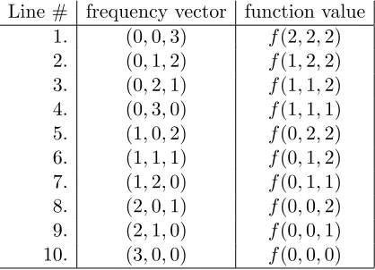
The truth table. We arrange the truth table of n+cn−1rows in lexicographic order. For example, forn=c= 3 we would have the following table:
Line # frequency vector function value
1. (0,0,3) f(2,2,2)
2. (0,1,2) f(1,2,2)
3. (0,2,1) f(1,1,2)
4. (0,3,0) f(1,1,1)
5. (1,0,2) f(0,2,2)
6. (1,1,1) f(0,1,2)
7. (1,2,0) f(0,1,1)
8. (2,0,1) f(0,0,2)
9. (2,1,0) f(0,0,1)
10. (3,0,0) f(0,0,0)
P1 must send to P2 the reduced truth table where the entries that are inconsistent with P1’s input are removed. That table encodes exactly the truth table of the residual function f(xi,·,·). Clearly, the reduced table also encodes a symmetric function over Zc = Z3, this time with only n−1 = 2 inputs. Moreover, whenP1 removes the inconsistent entries we get the truth table of the residual function again ordered by lexicographic order, no matter what was P1’s input. HenceP2 can continue by again removing the entries that are inconsistent, with his input without having to know which rows were removed by P1.
One way to see this visually is to imagine the following procedure that P1 employs for reducing the truth table: on input x1 = i ∈ Zc, P1 first subtracts one from the i’th coordinate in each entry of the frequency-vector column (to account for the fact that the input xi =i will be hard-wired in the residual function and should not be counted anymore), and then removes the rows corresponding to entries with negative numbers. (These are the inconsistent rows: since P1 has input i then consistent frequency-vectors couldn’t have zero in the i’th position.) An illustration of this transformation for the cases where P1’s input is x1 = 0 and x1 = 1 can be found below:
1. (0,0,3) 2. (0,1,2) 3. (0,2,1) 4. (0,3,0) 5. (1,0,2) 6. (1,1,1) 7. (1,2,0) 8. (2,0,1) 9. (2,1,0) 10. (3,0,0)
| {z }
original table
1. (−1,0,3) 2. (−1,1,2) 3. (−1,2,1) 4. (−1,3,0) 5. ( 0,0,2) 6. ( 0,1,1) 7. ( 0,2,0) 8. ( 1,0,1) 9. ( 1,1,0) 10. ( 2,0,0)
⇒
5. (0,0,2) 6. (0,1,1) 7. (0,2,0) 8. (1,0,1) 9. (1,1,0) 10. (2,0,0)
| {z }
x1=0
1. (0,−1,3) 2. (0, 0,2) 3. (0, 1,1) 4. (0, 2,0) 5. (1,−1,2) 6. (1, 0,1) 7. (1, 1,0) 8. (2,−1,1) 9. (2, 0,0) 10. (3,−1,0)
⇒
2. (0,0,2) 3. (0,1,1) 4. (0,2,0) 6. (1,0,1) 7. (1,1,0) 9. (2,0,0)
| {z }
x1=1
Note that in both cases the reduced truth table has entries with the same set of indexes. Therefore each subsequent party can apply a similar procedure to the table based on its own input, until the server obtains a table containing a single entry with the output of the function.
4.3 A Protocol for The Sum Function
We saw in Section 2.1 that the sum function f(x1, . . . , xn) = Pn
j=1xj has a simple minimum-disclosure decomposition. As we will see now, it also has a very simple optimally-private protocol. Note that this protocol works even in the case that the domain of the inputsxj is large (and thus the protocol for symmetric functions over Zccannot be used).
The semi-honest case. The protocol uses additively homomorphic encryption over the same group in which we compute the summation. The first party choosesn−1 random stringsr1,2, . . . , r1,n and encrypts the valuex+Pn
j=2r1,j under a public keypkS that was chosen by the server. It also encrypts each r1,j under the public-key pkj of the jth party Pj; denote c∗1 = EpkS(x+
Pn j=2r1,j) and c1,j =Epkj(r1,j). Next, when partyPj contacts the server, it receives the ciphertexts c
∗
j−1 and ci,j for i ≤ j, decrypts the ciphertexts ci,j in order to obtain the ri,j’s. Party j chooses random rj,k’s fork > j and addsxj−
P
i<jri,j+
P
It is possible to implement this using Paillier’s encryption [21]; this results in computing the sum modulo N. If it is necessary to compute the sum over the integers, then one simply needs to take N to be larger than n·L where (the absolute value of) each parties’ input is an integer between 0 andL. Alternatively we can use LWE-based schemes that can be made additively homomorphic over any group Zc, e.g. [10]. (In this case we must take care to ensure that the distributions of evaluated ciphertexts do not leak information.)
PROTOCOL 4.6. (Semi-Honest Optimal Protocol for the Sum Function)
• Inputs: Each partyPi (1≤i≤n) has a private inputxi, its own private keyski, and a
vector of public keys (pk1, . . . , pkn, pkS); the serverPn+1 has (pkS, skS) and (pk1, . . . , pkn).
LetDbe the domain of the homomorphic encryption scheme with public key pkS.
• The protocol:
1. Initialization: Letc∗0be an arbitrary encryption of zero under the Server’s public key.
2. Interaction of clientsP1, . . . , Pn with the server: For everyj= 1, . . . , n:
(a) The serverPn+1 sends toPj the ciphertextsc∗j−1 and all the ci,j’s fori < j. (If
j = 1 thenP1 can computec∗0on its own and theci,j’s are an empty list.)
(b) For all i < j, PartyPj decrypts ci,j with its own secret key,ri,j←Decskj(ci,j).
It also chooses a random rj,k fork=j+ 1, . . . , n+ 1 and encrypts it under the
key of Party Pk,cj,k←Encpkk(rj,k).
Let sj−1 be the value encrypted in c∗j−1. Party j then uses the homomorphic
properties with public key pkS to compute c∗j as an encryption of sj =sj−1+ xj−Pi<jri,j+Pk>jrj,k.
(c) PartyPj sends back toPn+1 the ciphertextsc∗j and all thecj,k’s fork > j.
3. Concluding the computation: Pn+1 decryptsc∗n+1 and outputs the value.
The malicious case. As in Protocol 4.2, we need to make sure that each party behaves cor-rectly. First, we need to ensure that the server’s public key was generated correctly (to ensure that the homomorphic operations truly hide each parties’ individual input). This can be carried out efficiently and non-interactively using [3]. Next, we need to make sure that each party updates c∗j correctly. This is a proof that two sums of ciphertexts (under different keys) are equal, which for Paillier’s encryption could be rather expensive. Finally, we need to know the secret key skS of the server (in case it is corrupted) in order to learn the new encrypted value (and the difference) thereby defining eachxj. However, this is already obtained via the proof in [3]. As in Protocol 4.4, the parties all also sign on their messages and proofs, and all of these are verified.
4.4 The Selection Functions
The semi-honest case. Our protocol is similar to the following 1-out-of-N (semi-honest) obliv-ious transfer protocol, using additively homomorphic encryption: The receiver, who wants to get the j’th value, generates N ciphertexts, all encrypting 1 except the j’th that encrypts a 0. Using the additive-homomorphism, the sender multiplies the ciphertexts by random numbers (a different random number for each ciphertext) and then adds his value xi to the i’th ciphertext. When the receiver decrypts, it gets thej’th value intact and all other values are random.
Our setting is a little more complicated than the OT setting, since (a) the inputs are split between parties P2, . . . , Pn rather than all belonging to one sender, and (b) the receiver in our case is the server Pn+1, while the selection index j is known to the first party P1. The latter concern is handled by choosing an encryption scheme with plaintext space much much larger than the domain of inputs to the parties. Now with high probability the j’th entry will be the only one in the domain of inputs, so the server can identify it.5 To handle the first concern we will use a mix-net-like construction (using a layer-rerandomizable ecnryption), with each party shuffling the ciphertexts so that the following parties cannot tell which ciphertext came from what party. (Also, we use El Gamal which is multiplicative- rather than additive-homomorphic, so we modify the underlying OT protocol accordingly.)
In more detail,P1with selector inputjprepares a vector of El Gamal ciphertexts, all encrypting the group generator G except the j’th that encrypts the group element 1. Thei’th ciphertext in this vector is encrypted under the compound El Gamal public keyHi,n+1 =Qn+1
t=i ht. (When using a generic layer-rerandomizable encryption, the i’th ciphertext is encrypted onion-style under the public keys of parties ithough n+ 1.) We call this vector the “initial ciphretexts” and denote it by I. During the protocol the initial ciphertexts will be passed unchanged, and the parties use them to process another vector of ciphertexts that contain the actual values. We call that other vector of ciphertexts the “work ciphertexts”, and denote it byW.
Each partyPi (i≥2) gets the initial ciphertextsI and a vectorWi−1 of i−2 ciphertexts. The ciphretexts in W are all encrypted underHi,n+1. Pi takes thei’th ciphertext fromI (which is also encrypted underHi,n+1), uses the multiplicative homomorphism of El Gamal to raise the plaintext inside it to a random power inZq, then uses the homomorphism again to multiply the plaintext by its input xi. It inserts the resulting ciphertext toWi−1, thus getting a vecotr ofi−1 ciphertexts which we denote by Wi0. Pi then peels off its layer of encryption (resulting in ciphertexts under Hi+1,n+1), randomly permutes the ciphertxts and re-randomizes them, thus obtaining a new vector of ciphertexts Wi, which Pi sends back to the server.
After all the players participated, the server has a vector of “work ciphertexts” Wn, encrypted under the public key of the server Hn+1 = hn+1. The server decrypts this vector, and if the corresponding plaintext vector has a single element from the input domain of the protocol then the server outputs that element. A pseudocode description of this protocol (described using a generic additively homomorphic encryption layer-rerandomizable) can be found in Protocol 4.7.
Using similar arguments as in the binary symmetric case, we have that Protocol 4.7 is optimally-private in the presence of augmented semi-honest adversaries, if the encryption schemes used is addi-tively homomorphic and layer rerandomizable, and has plaintext space which is super-polynomially larger than the input space for the protocol.
An error-free variant. The small probability probability of error in the protocol above can be easily removed. If the input space for the protocol is some Zc, then we choose encryption scheme
PROTOCOL 4.7. (Semi-Honest Optimal Protocol for the Selection Function) • Inputs: PartyP1has an indexj (2≤j≤n), and each partyPi (2≤i≤n) has a private
inputxi, its own private keyski, and a vector of public keys (pk2, . . . , pkn, pkn+1).
• The protocol:
1. First party instructions:
(a) For every i = 2, . . . , n, i6= j, P1 computesci = ¯Epki,...,pkn+1(1). Fori =j, P1 computescj = ¯Epkj,...,pkn+1(0).
(b) P1 sends the vector of initial ciphretextsI = (c2, . . . , cn) to the serverPn+1.
2. Interaction of clientsP2, . . . , Pn with server. Fori= 2, . . . , n:
(a) Pn+1 sendsPi the initial ciphertexts I, and a vectorWi−1 of i−2 ciphertexts,
encrypted underpk~i= (pki, . . . , pkn+1). (Fori= 2, W1is empty.)
(b) Pi extracts the i’th ciphretext from I, ci = I[i] (encrypting a bit bi ∈ {0,1}
under pk~i.) It chooses a random number ri from the plaintext space and uses
the encryption additive-homomorphism to compute a ciphertextc0i=ricixi,
encrypting the plaintext valueri·bi+xi.
(c) Pi addsc0i to the vectosWi−1 (thus receiving a vector ofi−1 ciphertexts under
(pki, . . . , pkn+1)) and decrypts a layer of all of these ciphertexts using its secret
keyski; denote the result by Wi0.
(d) Pipermutes the ciphertexts inWi0and rerandomizes all of them using the public
keyspki+1, . . . , pkn+1. Denoting the result byWi,PisendsWiback to the server.
3. Concluding the computation: Upon receiving the encrypted vectorWn(of lengthn−1)
fromPn, the serverPn+1 decrypts all the ciphertext using its secret keyskn+1. If the
corresponding plaintext vector includes a single element from the input space then the server outputs that plaintext (else it outputs ‘?’).
with plaintext space that includesZc+1 ={0,1, . . . , c}. Then partyPi (i≥2) with inputxi ∈Zc, instead of choosing ri at random as above smiply setsri =c−xi. This ensures that the value that the server recovers is eitherxi (ifPi received an encryption of 0) orc (ifPi received an encryption of 1).
The malicious case. As above, in this case we need to have the parties prove that they behaved honestly. This can be achieved using similar techniques as those described above.
5
Securely Computing any Decomposition
We now turn to the task of securely computing an arbitrary given decomposition. For this we use
re-randomizable garbled circuits that were introduced by Gentry et al. for the purpose of multi-Hop homomorphic encryption [11]. (Below we call this the GHV construction.) Very roughly, each party i receives from the server a garbled circuit encoding ˜fi−1(x1, . . . , xi−1), adds its input to generate a garbled circuit for ˜fi(x1, . . . , xi), then re-randomizes this garbled circuit (so as to hide xi from colluding dishonest partiesi−1 andi+ 1) and sends the result back to the server.
the adversary to be able to evaluate ˜fj for any j < i. (In contrast, in the setting of multi-Hop homomorphic encryption if party i+ 1 is dishonest then the adversary can evaluate ˜fi.)
To solve this we again use layered re-randomizable encryption: instead of giving the players the input labels for the garbled circuit, we give them only the encryption of these input labels, encrypted under all the keys of of the parties that did not participate yet. Each party peels of its layer of encryption and re-randomizes the result, hence the server learns the input label only after all the (honest) parties decrypted their layers, and it cannot evaluate the circuit earlier.
We note that the layered re-randomizable encryption is intertwined with the garbled-circuit construction, since each party has to be able to transform the encryption of the inputs of one garbled circuit into “freshly random” encryption on the inputs to a re-randomized version of the garbled circuit. Recall that in the GHV construction the labels on the wires are balanced bit-strings (with half 0s and half 1s), and re-randomizing a circuit is done by bitwise permuting the labels. Hence we use bit-wise encryption (to handle the permutation) where ciphertexts can be re-randomized (to hide the correlation to the previous circuit).
The GHV construction is described in Section 5.1. We mention that the original construction from [11] is secure only in the semi-honest model. In particular a malicious party can choose “bad labels” to wires to foil re-randomization, by choosing the two labels on a wire with a very small (or very large) Hamming distance. We thus modify the construction slightly and require that the Hamming weight between the two labels be exactly half their length. This turns the GHV construction into one that works for any adversarial coins in the semi-honest model, so we can add (non-interactive) zero-knowledge proofs and get resilience against malicious adversary.
5.1 The GHV Construction
The GHV construction works over an algebraic group of prime order q where the decision Diffie-Hellman assumption is believed to hold. The labels on the wires of garbled circuits are of length `= 3|q| (and we assume for convenience that ` is divisible by 4). A Boolean circuit is garbled by choosing two random `-bit labels, each with Hamming weight exactly `/2, and in our variant also with Hamming distance exactly`/2 from each other. One way to choose such labels is to start with the labels L0∗ = 0`/21`/2 and L1∗ = 0`/41`/40`/41`/4, and then chose a random bit permutation π and apply it to both L0∗, L1∗, setting L0 =π(L0∗) and L1 =π(L1∗).
Given the labels on all the wires, a gate is represented by four pairs of ciphertexts under the (bit-by-bit version of the) BHHO cryptosystem [2], one pair for each line in the truth table of the gate. Let R0, R1 be the two labels on the first input wire, S0, S1 be the two labels on the second input wire, and T0, T1 be the two labels on the output wire of the gate. For a line (a, b) 7→ c in the truth table (with a, b, c ∈ {0,1}), we choose at random r, r0 ∈ {0,1}` such that r⊕r0 = T c,
and encrypt r under Raand r0 underSb, thus forming the pair (EncRa(r),EncSb(r0)). The gate is represented by the four pairs of ciphertexts in random order.
In addition, for the purpose of re-randomization we include with each ciphertext EncL(r) also the BHHO public key corresponding to the secret key L. The same public keys can be used also to identify the right ciphertext-pair to decrypt when evaluating the garbled circuit: If we know the two input labelsRa, Sb for some gate, then we decrypt the ciphertext-pair that includes the public keys corresponding to these two labels.
BHHO public keyspk(L0) and pk(L1) in order. Upon evaluation, we output 0 if the output labels that we learn corresponds to the first public key and 1 if it corresponds to the second. (We note that these public keys allow one to extend the garbled circuit, since to generate EncL(r) it is sufficient to knowpk(L) and we don’t need to know Lexplicitly.)
Re-randomization of a circuit is done as follows:
1. Choose a random bit permutation πw over [`] for every wirew in the circuit. If the labels on that wire areL0w, L1w then the new labels will beπw(L0w), πw(L1w), respectively.
2. Use the BHHO key- and plaintext-homomorphism to translate each ciphertext EncL(r) into
Encπ(L)(π0(r)) according to the permutations from Step 1. Also transform similarly all the attached public keys from pk(L) to pk(π(L)).6
3. For each ciphertext-pair (EL(r), EL0(r0)), choose a random δ ∈ {0,1}` and use the BHHO
plaintext homomorphism to transform the pair into (EL(δ⊕r), EL0(δ⊕r0)).
4. Using the attached public keys, re-randomize all the BHHO ciphertexts and public keys, thus getting new (pseudo)random ciphertexts and public keys for the new labels.7
Let us denote by Λf = GC(f, r) the garbled circuit for circuit f that was generated using the randomnessr, and by Λ0f = ReRand(Λf, r∗) the re-randomized circuit that was generated from Λf using randomnessr∗. The next lemma asserts that Λ0f results is (pseudo)random, even conditioned on the randomnessr.
Lemma 5.1. If the decision Diffie-Hellman problem is hard in the group underlying the GHV construction, then for every fixed circuit f and randomness r, the following two distributions are computationally indistinguishable:
Dfresh def
=
(f, r,Λ0f) : r0 is fresh randomness,Λ0f = GC(f, r0) , and
DreRnd def=
(f, r,Λ0f) : r∗ is fresh randomness,Λf = GC(f, r),Λ0f = ReRand(Λf, r∗)
Proof (sketch). This lemma was essentially proved in Theorem 7 of Gentry et al. [11] (Theorem 8 in the full version). The only difference is that it was only proved for randomly chosen r, not every r as stated above. The reason is that the GHV permutation lemma from [11] only applies when the two labels on a wire are chosen at random. We note however that the proof of that lemma goes through as long as the two labels on each wire have Hamming distance close to `/2 (and the only use of the randomly-chosen labels is to argue that their Hamming distance is indeed close to `/2). In our version of the construction the distance between the two labels is always exactly`/2, regardless of the randomness used. Hence we get the stronger statement of Lemma 5.1.
5.2 Our Construction, Semi-Honest Model
As described above, we get security in our model by augmenting the GHV construction with encryption of the input labels. Differently from Gentry et al., we do not use oblivious transfer to
6
BHHO public keys are just encryptions of 0, so every operation that can be applied to ciphertexts can also be applied to public keys.
7By pseudorandom we mean that they cannot be distinguished from fresh random ciphertexts (or public keys)