Milder Definitions of Computational Approximability: The Case of Zero-Knowledge Protocols

(1)

Milder Definitions of Computational

Approximability: The Case of Zero-Knowledge

Protocols

Mohammad Sadeq Dousti and Rasool Jalili

Abstract—Many cryptographic primitives, such as pseudorandom generators, encryption schemes, and zero-knowledge proofs, center around the notion ofapproximability. For instance, a pseudorandom generator is an expanding function which on a random seed,approximatesthe uniform distribution. In this paper, we classify different notions of computational approximability in the literature, and provide several new types of approximability. More specifically, we identify two hierarchies of computational approximability: The first hierarchy ranges fromstrongapproximability—which is the most common type in the cryptography—to the

weakapproximability—as defined by Dworket al.(FOCS 1999). We define semi-strong, mild, and semi-weak types as well. The second hierarchy, termedK-approximability, is inspired by theε-approximability of Dworket al.(STOC 1998).K-approximability has the same levels as the first hierarchy, ranging from strongK-approximability to weakK-approximability. While both hierarchies are general and can be used to define various cryptographic constructs with different levels of security, they are best illustrated in the context of zero-knowledge protocols.

Assuming the existence of (trapdoor) one-way permutations, and exploiting the random oracle model, we present a separation between two definitions of zero knowledge: one based on strongK-approximability, and the other based on semi-strongK -approximability. Especially, we present a protocol which is zero knowledge only in the latter sense. The protocol is interesting in its own right, and can be used for efficient identification. Next, we show that our model for zero knowledge wasnotclosed under sequential composition, and change the model to resolve this issue. After proving a composition theorem, we finally provide a version of the identification protocol which satisfies the requirements of the new model. Some techniques provided in this paper are of independent interest, such as proving a composition theorem in the presence of both simulator and knowledge extractor.

Index Terms—Interactive and reactive computation, Probabilistic computation, Network-level security and protection, Authentica-tion, Cryptographic controls.

F

1 I

NTRODUCTION

The notion ofcomputational approximabilitycan be tracked down to works such as [1], [2], [3], [4], [5], [6], but it was probably the work of Goldwasser, Micali, and Rackoff on zero-knowledge proofs [7, Section 3.2] which explicitly defined the notion. Informally, the output of a probabilistic machine is said to approximate a random variable if no polynomial-size circuit can tell them apart. All works which use the notion of indistinguishabilitycan be reformulated to use the notion ofapproximabilityinstead. For instance, pseudorandom generators, encryption schemes, and witness-hiding proofs can all be defined in terms of approximability. However, approximability is best illustrated in the context of zero-knowledge protocols. In fact, our research on approximability was initiated while we were exploring less strict models of zero knowledge.

Let us explain the motivation behind the need for looser models of zero knowledge: Over time, some authors proved inherent limitations to the accepted notions of zero-knowledge proofs, most of which were imposed on the round complexity of the proof. For instance, Goldreich, Oren, and Krawczyk [8], [9] proved lower bounds on the

• M.S. Dousti and R. Jalili are with the Department of Computer Engineering, Sharif University of Technology, Tehran, Iran.

E-mail:{dousti@ce., jalili@}sharif.edu

round complexity of auxiliary-input and black-box zero-knowledge proofs (with negligible soundness error). To overcome these and similar limitations, less strict models of zero knowledge was suggested. To name just a few examples, Brassardet al. [10] put forward the notion of arguments, Barak [11] advocated a non–black-box model of zero knowledge, Dwork and Stockmeyer [12] proposed a model where the prover’s resources were limited, Pass [13] suggested permitting the simulator to run in quasi-polynomial time, and Birrell and Vadhan [14] modeled the verifier as circuits with bounded non-uniformity.

Most relevant to the present work, several researchers argued that the current formulation of approximability is too strong for some purposes, and consequently proposed weaker notions of approximability. For instance, Dwork, Naor, Reingold, and Stockmeyer [15], [15] proposed the notions of weak and ultra-weak approximabilities.1Let us intuitively compare the current formulation of approximability (which we termed “strong approximability”) with the weak variant defined by Dwork et al.: Suppose M is a probabilistic polynomial-time machine which is going to approximate a distribution ensemble{U(x)}indexed by some set L(i.e.

x∈L).

(2)

1) In strong approximability, M should approximate

{U(x)}, such that the output ofM(x)is indistinguish-able fromU(x) by all polynomial-size testsD. 2) In weakapproximability, the code ofM may depend

on bothxandD, as if we say: Disclose the index and the test, and we will exhibit an approximator which beats the test.

The security guarantees provided by the weak approx-imability is way too low, as M can arbitrarily depend on the code of the adversary. As a matter of fact, weak approximability was not introduced to serve security pur-poses at all. Therefore, we sought milder notions of approximability, which provide better security guarantees than the weak approximability, yet are not as strict as the strong approximability.

More specifically, we consider a hierarchy of successive weakenings of approximability, and put forward three notions of semi-strong, mild, and semi-weak approximabil-ities. Intuitively, the semi-strong variant assumes that the approximator has black-box access to the distinguisher. Mild approximability requires a universal approximator which may receive the description of the distinguisher as an auxil-iary input. Finally, the semi-weak approximability allows the approximator to depend arbitrarily on the distinguisher, but not the index (x).

The security guarantees of the semi-strong approximation is still very high: It does not seem that the one-bit output of the distinguisher is of much help to the approximator.2 The same holds for the mild approximability: Unless the approximator can “reverse engineer” the description of the distinguisher, it cannot gain insight significantly better than an approximator which merely has black-box access to the distinguisher. That said, we successfully exhibit a separation between the strong and semi-strong approximations in the random-oracle model, assuming the existence of (trapdoor) one-way permutations.

Another hierarchy of approximability is inspired by the work of Dwork, Naor, and Sahai [18], [19]. Failing to demonstrate a concurrent zero-knowledge proof with low round complexity (due to some inherent limitations), they promoted a new definition which we termε-approximability. In this definition, the running time of the approximator can be a polynomial in the running time of the distinguisher, as well as the inverse of the distinguishing gap (ε−1_).

Applying the same ideas, we provide another hierarchy termedK-approximability, whose levels range from strong

K-approximability to weakK-approximability. This hier-archy combines approximators with knowledge extractors, and is somehow weaker than the previous hierarchy. The aforementioned separation actually separates strong and semi-strongK-approximabilities.

2. It must be noted, though, that the importance of a single bit should not be underestimated. For instance, a single bit of advice can help compute some uncomputable functions [16, Theorem 1.13]. That said, it is hard to conceive of a natural problem in which the one-bit output of the distinguisher is of much help to the approximator (see [17]). In fact, even this paper does not use the one-bit output of the distinguisher; rather, it uses the random-oracle model to force the distinguisher make some queries, and then monitors them.

The ideas and techniques offered by this paper might be of independent interest, among them is an efficient identifica-tion protocol used to separate two noidentifica-tions of approximability, and a new technique for proving a composition theorem in the presence of both simulator and knowledge extractor.

1.1 Motivation

A natural question that may arise is why we weaken the existing definitions. There are several answers to this question:

1) The new definitions are not weaker than all the existing ones; rather, they are stronger than definitions like the

weakandultra weak zero knowledgedefined by Dwork

et al. [20]. The weak definitions never found their way into the practice, because the community felt that they are inadequate for everyday protocols and applications. However, such weak definitions are important to the theorists, as they are related toselective commitment

andmagic functions (see [20] for more information). This paper provides definitions which aremilder than the existing ones, i.e. they are stronger than some existing definitions, and weaker than other ones. They might bridge the gap, and provide models which are of interest to both theorists and practitioners.

2) Before the introduction of the notion ofwitness-hiding proofs [21], no formal proof for the security of the parallel version of Feige-Fiat-Shamir identification protocol [22] was available. However, the security guarantee of being “witness hiding” is much weaker than being “zero knowledge.” Consequently, it is desirable to have definitions based on which a tighter security guarantee is possible. Therefore, weakening strong definitions of zero knowledge is desirable in some cases.

As a matter of fact, we were able to prove the security of efficient identification protocols (see Protocols 1 and 3) in a rather tight manner. According to previous definitions, these protocols were either deemed insecure, or their security were proven in a loose manner. 3) As discussed in Section 6, the new definitions shed

light on an alternative way of replacing a random oracle with a new, suitable cryptographic assumption.

1.2 Organization

(3)

2 P

RELIMINARIES

2.1 Notions and Abbreviations.

LetN={0,1,2, . . .}denote the set of natural numbers. For

a languageLand a numbern∈_N, defineLn def

=L∩{0,1}n_. The expected value of a random variableX is denoted by

E[X]. We use the quantifier∀∞ as a shorthand for “for all

but finitely many.” For instance,(∀∞_n_∈

N)[ϕ(n)]means

“for all but finitely many natural numbersn, the predicate

ϕ(n) holds.” Formally, (∃n0 ∈ N)(∀n ∈ N)[n ≥ n0 ⇒

ϕ(n)].

Throughout the paper, we use the following abbreviations: RO and ROM are stand for “random oracle” and “random-oracle model.” TM stands for Turing machine, PPT for probabilistic polynomial-time, PPTM for a PPT TM, ITM for interactive Turing machine, and OM for oracle machine. These terms might be combined together; for instance, PPT-OM means a “probabilistic polynomial-time oracle machine.” We also use “ZK” for zero knowledge. To denote the type of ZK (see Section 2.2), we use prefixes such as AI (auxiliary input) and BB (black box). Therefore, AIZK means “auxiliary-input zero knowledge.”

A family of circuitsC={Cn} is calledpolynomial-size if there exist polynomials p(·) and q(·) such that for all

n∈N, the size and the number of inputs ofCnare bounded byp(n)and q(n), respectively. We assume that all circuits are probabilistic.

2.1.0.1 Convention.: When we say a machine is polynomial-time, we mean polynomial in the length of itsfirst input. We may “pair” two or more inputs and feed them as the first input to a machine. For instance, the first input toM(hx, y, zi, w, t)ishx, y, zi. The same convention holds for polynomial-size circuits.

2.2 Definitions

Definition 1(Trapdoor One-way Permutation). A family of permutationsF={fn} is called acollection of trapdoor

one-way permutations if there exist four PPT algorithms GEN, SAMP, EVAL, and INV, such that the following conditions hold:

1) Easy to generate: On input 1n_{, algorithm GEN} generates a description of fn denoted desc(fn), as well as the associated trapdoortn. Denote the first (i.e.

desc(fn)) and second (i.e.tn) components in the output of GEN by GEN1 and GEN2, respectively. In order to

avoid mentioning 1n explicitly in the inputs of SAMP, EVAL, and INV, we assume that |desc(fn)| ≥n. 2) Easy to sample the domain: On input desc(fn),

algorithm SAMP chooses an element fromdom(fn). 3) Easy to evaluate: On inputs desc(fn) and x ∈

dom(fn), the output of the algorithm EVAL isfn(x). 4) Easy to invert with trapdoor: On inputs desc(fn),

tn, andy∈dom(fn), the output of the algorithm INV is fn−1(x). (Note that since fn is a permutation, its range is identical to its domain.)

5) Hard to invert without trapdoor:For every family of polynomial-size circuits A={An}, for every c∈N,

and for all sufficiently large n:

Prhdesc(fn)←GEN1(1n),

x←SAMP(desc(fn)),

y←EVAL(desc(fn), x) :

An(y,desc(fn)) =x

i

< n−c ,(1) where the probability is taken over the random coins of GEN, SAMP, EVAL, andA.

Definition 2 (Strong Approximability). A polynomially-bounded distribution ensemble3 _{_U₍_{x, z}₎_}

x∈L,z∈{0,1}∗ is

said to be strongly approximable on the language L, if there exists a PPTMM(·,·)such that for every family of polynomial-size circuitsD={Dn}, the following holds:

(∀c∈N)(∀∞n∈N)(∀x∈Ln)(∀z∈ {0,1}∗)

|Pr[Dn(x, z, M(x, z)) = 1]−

Pr[Dn(x, z, U(x, z)) = 1]|< n−c , (2) where the first probability is taken over the random coins ofM andDn, and the second probability is taken over the (implicit) random coins ofU andDn.

Let hP↔V∗(z)i(x) be a protocol between ITM P and PPT-ITM V∗, where the common input is x and V∗

has an auxiliary input z. Define viewV∗ =def view_V∗(x,

z)=defviewV∗hP ↔V∗(z)i(x)as whateverV∗ sees during

the interaction withP; that is, the common input (x), the auxiliary input (z), its random tape (r), and the messages it sent and receivedm= (m1, m2, . . .).

Definition 3 (Auxiliary-Input Zero Knowledge (AIZK)).

The protocol hP↔V∗(z)i(x)is AIZK forP on Lif for all PPTMV∗, there exists a PPTM simulator SV∗ which strongly approximatesthe view ofV∗. That is, for every family of polynomial-size circuitsD={Dn}, the following holds:

(∀c∈_N)(∀∞_n_∈

N)(∀x∈Ln)(∀z∈ {0,1}∗)

|Pr[Dn(x, z, SV∗(x, z)) = 1]−

Pr[Dn(x, z,viewV∗(x, z)) = 1]|< n−c , (3)

where the first probability is taken over the random coins ofSV∗ andDn, and the second probability is taken over

the random coins ofP,V∗ andDn.

Throughout the paper, we are mostly concerned with the notion of “zero knowledge” rather than the notion of the “proof.” Therefore, we hardly mention properties such as completeness and soundness, even if the zero-knowledge protocols provide them. Moreover, while the definitions resemble proofs of language membership [7], they can be applied to proofs of knowledge [23] or proofs of computational ability [24] as well.

(4)

3 T

WO

H

IERARCHIES OF

A

PPROXIMABILITY

3.1 The First Hierarchy

Let us first present the notion of weak approximability, inspired by theweak zero-knowledge definition of Dwork

et al. [15], [20]:4

Definition 4 (Weak Approximability). A poly-bounded distribution ensemble U ={U(x, z)}x∈L,z∈{0,1}∗ is said

to beweakly approximableon the languageL, if for every family of polynomial-size circuitsD={Dn}, the following holds:

(∀c∈N)(∀∞n∈N)(∀x∈Ln)

(∀z∈ {0,1}∗)(∃M ∈PPTM)

|Pr[Dn(x, z, M(x, z)) = 1]−

Note that in Definition 4, the machine M can depend on x, z, and Dn, as well as U. It can be symbolized as (∀D)(∀∞_x _∈ _L₎₍_∀_z₎₍_∃_M_)[_D₍_{x, z, M}₍_{x, z}₎₎ _≈ _D₍_x,

z, U(x, z))], which is interpreted: “You name the test (Dn) and the parameters (x,z), and I will present a machine (M) which approximates U in such a way that the test fails.”

Remark 1. A natural but misleading question is the fol-lowing: “In the real world, how can the approximator access the distinguisher?” The important point is that neither approximator nor the distinguisher are real-world

entities; they are just parts of a thought experiment. The right interpretation is the following: Consider a real-world entity who uses some (internal) procedure to distinguish the distributions. This entity can modify the procedure to produce the right distribution.

The weak approximability seems to be extremelyloose, and it is natural to think of a tighter notion. One such attempt is made in Definition 5.

Definition 5 (Semi-Weak Approximability). A poly-bounded distribution ensembleU ={U(x, z)}x∈L,z∈{0,1}∗

is said to besemi-weakly approximableon the languageL, if for every family of polynomial-size circuits D={Dn}, the following holds:

(∀c∈N)(∀∞n∈N)(∃M ∈PPTM) (∀x∈Ln)(∀z∈ {0,1}∗)

|Pr[Dn(x, z, M(x, z)) = 1]−

4. It must be noted, though, that their definition is based on the uniform zero knowledge [25].

Definition 5 allowsM to depend onDn, but not on x

orz. It can be interpreted as “You name the test (Dn), and I will present a machine (M) which approximates U in such a way that the test fails.” This is still too loose:M is effectively a circuit, not a PPTM. This is becauseM can depend on the non-uniformity ofDn, and access the same (or even longer) prefix of z thatDn does.

One way to restrain this power is not to allow M to depend onDn arbitrarily. To this end, we require that there exists some universal PPTMM which can approximateU

onL, but we letM to havecode accessorblack-box access

toDn. Definitions 6 and 7 capture the new notions:

Definition 6 (Mild Approximability). A poly-bounded distribution ensembleU ={U(x, z)}x∈L,z∈{0,1}∗is said to

bemildly approximable on the languageL, if there exists a PPTMM, such that for every family of polynomial-size circuitsD={Dn}, the following holds:

(∀c∈N)(∀∞n∈N)(∀x∈Ln)(∀z∈ {0,1}∗)

|Pr[Dn(x, z, M(hx,desc(Dn)i, z)) = 1]−

Pr[Dn(x, z, U(x, z)) = 1]|< n−c , (6) where the first probability is taken over the random coins of M and Dn, and the second probability is taken over the (implicit) random coins ofU andDn. Here,desc(Dn) means the description of the circuitDn in some canonical encoding.

Note that since the pair hx,desc(Dn)i is provided as the first input toM, the machine M has enough time to simulate the code ofDn.

Definition 7 (Semi-Strong Approximability). A poly-bounded distribution ensembleU ={U(x, z)}x∈L,z∈{0,1}∗

is said to besemi-strongly approximableon the languageL, if there exists a PPT-OMM, such that for every family of polynomial-size circuitsD={Dn}, the following holds:

(∀c∈N)(∀∞n∈N)(∀x∈Ln)(∀z∈ {0,1}∗)

|Pr[Dn(x, z, MDn(x, z)) = 1]−

The interpretation of Definition 6 is: “I will provide an approximator M that, given the code of the test, will approximateU onLsuch that the test fails.” Definition 7 is interpreted similarly; yet instead of accessing the description of the test, the machineM is only allowed black-box access to the test.

Theorem 1. Let us denote the “entailment” by⇒. Then: Strong approximability⇒Semi-strong approximability⇒

Mild approximability ⇒ Semi-weak approximability ⇒

Weak approximability.

(5)

can have black-box access to the distinguisher. If the approximation is possible without such access (as is the case with strong approximability), it isa fortioripossible with black-box access.

The same reasoning holds while comparing semi-strong and mild approximabilities: If the approximation is possible with only black-box access (as is the case with semi-strong approximability), it isa fortioripossible with code access (as is the case with mild approximability).

Mild approximability implies semi-weak approximability since the order of quantifiers in the definition of the latter allows the approximator to dependarbitrarilyon the distinguisher.

Semi-weak approximability implies weak approximability because the latter allows the approximator to depend not only on the distinguisher, but also on the common and auxiliary inputs.

It is easy to take cryptographic primitives which incorpo-rate “strong approximability” and redefine them based on the new notions of approximability. For instance, consider the definition of “pseudorandom generators”: Let`(n)> nbe a polynomially-bounded function. The functionG:{0,1}n _→

{0,1}`(n) _{is called a pseudorandom generator if it is}

polynomial-time computable, and for a randomly selected

x ∈ {0,1}n_{, the uniform distribution over} _{₀_,₁_}`(n) _is

strongly approximated byG(x).5 _{It is now easy to define,} say, a “mildly pseudorandom generator”: The function

G is called a mildly pseudorandom generator if it is polynomial-time computable, and for a randomly selected

x ∈ {0,1}n_{, the uniform distribution over} _{₀_,₁_}`(n) _is mildly approximatedbyG(x).

Separating Definitions 4–7 from each other and from Definition 2, as well as determining the security implications each provides, seems to be an interesting task. Specifically, it seems hard to separate the semi-strong approximability (Definition 7) from the strong approximability (Definition 2). On the one hand, the approximator M of Definition 7 can perform tests based on the non-uniformity ofDn, something that a PPTM cannot do by itself. On the other hand, the one-bit output ofDn does not seem to offer machineM of Definition 7 any competitive advantage over the machine

M of Definition 2. However, in Section 4 we will see a separation between the strong approximability and the semi-strong approximability in the random-oracle model. (In fact, we provide such separation in the context of the second hierarchy; see below.)

3.2 The Second Hierarchy

The second hierarchy we present has more “semantics” attached to it. This hierarchy concerns theknowledgewhich might be encoded into the description of a distinguisher, or given as an external advice to it. The models in this hierarchy allow the approximator to extract the knowledge

5. The technicality here is that the selection ofxfromLis notuniversally quantified; instead,xisrandomlyselected from{0,1}n_{. One can easily}

change the definitions of approximability to cover this case as well.

associated with a particular distinguisher, and then try to approximate the distribution ensemble.

Informally, a TM/circuitD is said to know something with probability q if there exists a probabilistic TM K

(called the knowledge extractor), which runs in expected time bounded by to1/q (up to a polynomial factor), and extracts the knowledge ofD. The machine K may have black-box [22], [21], [23] or code access [26], [27] toD. Depending on how wellK extracts the knowledge, one can definestrong proofs of knowledge [28, Definition 4.7.13], (ordinary) proofs of knowledge [28, Definition 4.7.2], and

weakproofs of knowledge (an adaption of weak proofs of ability defined in [24]). The combination of {black-box, code} access, and{strong, ordinary, weak}models provide us with 6 possible ways of defining a hierarchy. Below we will present some natural combination; but let us provide an example first.

Consider a cryptographic protocol, such as an identifi-cation scheme. In this protocol, the proverP must prove his knowledge of some secrets(related to his identity) to a verifierV∗. Assume the protocol is defined in such way that it has a special behavior:6

1) UnlessV∗ “knows”s, she cannot distinguish the real execution from a simulated one.

2) IfV∗gets to “know”s, she might be able to distinguish the real and simulated executions.

The question is: “does the second case harm the security of the identification scheme?” After all, if the adversary knows the secret, she can simulate the protocol all by herself, without having to communicate with the prover. We may therefore present an informal definition ofsimulatable identification schemes, as below:

An identification scheme is simulatable if for every PPTM adversaryV∗, there exists a simulator

SV∗ which simulates the view ofV∗, in such a

way that if the adversary can distinguish the real and simulated views with probability q, we can conclude that she knows the secret of the prover with probability roughlyq.

This notion of simulatability is closely related to what Dwork, Naor, and Sahai [18], [19] calledε-knowledge, based on which one can define ε-approximability. However, in order to be consistent with the naming convention of the previous hierarchy, we call it “strong ε-approximability.”

Definition 8(Strongε-Approximability). A poly-bounded distribution ensembleU = {U(x, z)}x∈L,z∈{0,1}∗ is said

to bestronglyε-approximableon the language L, if for all functions0< ε(·) =o(1), there exists a PPTM M, such that for every family of polynomial-size circuitsD={Dn}, the following holds:

(∀c∈N)(∀∞n∈N)(∀x∈Ln)(∀z∈ {0,1}∗)

|Pr[Dn(x, z, M(hx,11/ε(n),|Dn|i, z)) = 1]−

(6)

where the first probability is taken over the random coins ofM andDn, and the second probability is taken over the (implicit) random coins ofU andDn.

Note that the running time of M can be a polynomial in the size of the distinguisher, as well as the inverse of the distinguishing gap (ε−1_{). For several years, it was}

unknown whether zero-knowledge is a stricter concept than

ε-knowledge. Barak and Lindell [27] showed a separation between the two concepts: While there exist constant-round strict polynomial-time black-box simulator ε-knowledge proofs for NP (with negligible soundness error), such constant-round strict polynomial-time black-box simulator ZK proofs (with negligible soundness error) exist only for

BPPlanguages.7

As in the previous section, it is possible to define the hierarchy of weak ε-approximability, semi-weak ε -approximability, mild ε-approximability, and semi-strong

ε-approximability. However, the goal of this section is to provide a different hierarchy based on the notion of knowledge extraction.

Recall the example about the identification scheme: It was designed such that if the adversary could distinguish the real and simulated executions with probabilityq, then it wouldknowthe secret of the prover with probabilityq. The word “know” is italicized because it is informal. One can formalize this definition by requiring the existence of a knowledge extractorK, such thatKaccesses the adversary, extracts her knowledge, andtries to simulate the protocol. Definitions 9 and 16 formalize this concept.

Definition 9 (MildK-Approximability). A poly-bounded distribution ensemble U ={U(x, z)}x∈L,z∈{0,1}∗ is said

to bemildly K-approximable on the languageL, if there exists a PPTMM and an expected PPTMK, such that for every family of polynomial-size circuits D = {Dn}, for all n∈N, for all x∈Ln, and for all z ∈ {0,1}∗, if the advantage

Ψn=AdvM,UDn (x, z)

def

=|Pr[Dn(x, z, M(x, z)) = 1]

−Pr[Dn(x, z, U(x, z)) = 1]| (9) is nonzero, then on input(x, z), the following holds:

|Pr[Dn(x, z, K(hx,11/Ψ,desc(Dn)i, z)) = 1]

−Pr[Dn(x, z, U(x, z)) = 1]|

< n−c , (10) where the first probability is taken over the random coins ofK and Dn, and the second probability is taken over the (implicit) random coins ofU andDn.

Definition 10(Semi-StrongK-Approximability). A poly-bounded distribution ensembleU ={U(x, z)}x∈L,z∈{0,1}∗

is said to besemi-stronglyK-approximableon the language

L, if there exists a PPTM M and an expected PPT-OM

K, such that for every family of polynomial-size circuits 7. A very recent treatment of this subject can be found in [29].

D = {Dn}, for all n ∈ N, for all x ∈ Ln, and for all

z ∈ {0,1}∗_{, if} _{Ψ =} _AdvM,U

Dn (x, z) (defined in (9)) is

nonzero, the following holds:

|Pr[Dn(x, z, KDn(hx,11/Ψi, z)) = 1]−

Pr[Dn(x, z, U(x, z)) = 1]|

< n−c , (11) where the first probability is taken over the random coins ofK and Dn, and the second probability is taken over the (implicit) random coins ofU andDn.

As in the first hierarchy, other levels of the

K-approximability (strong, semi-weak, and weak K -approximabilities) are conceivable as well (see the Ap-pendix).

Theorem 2. Each definition of approximability entails the corresponding variant ofK-approximability. Moreover,

Strong K-approximability ⇒ Semi-strong K -approximability⇒MildK-approximability ⇒Semi-weak

K-approximability ⇒WeakK-approximability.

Proof: In the definitions of K-approximability, the knowledge extractor has more freedom over the approxima-tor, since its running time may depend on the distinguishing advantage. Therefore, if some distribution ensemble is approximable, it isa fortiori K-approximable.

The entailments of this theorem can be proven similar to the proof of Theorem 1:

Strong K-approximability implies semi-strong K -approximability since, in the latter, the knowledge extractor (K) can have black-box access to the distinguisher. If the approximation is possible without such access (as is the case with strong approximability), it isa fortioripossible with black-box access.

The same reasoning holds while comparing semi-strong and mild approximabilities: If the approximation is possible with only black-box access (as is the case with semi-strong approximability), it isa fortiori possible with code access (as is the case with mild approximability).

Mild approximability implies semi-weak approximability since the order of quantifiers in the definition of the latter allows the knowledge extractor to dependarbitrarilyon the distinguisher.

Semi-weak approximability implies weak approximability because the latter allows the knowledge extractor to depend not only on the distinguisher, but also on the common and auxiliary inputs.

4 S

EPARATING

S

EMI

-S

TRONG

A

PPROXIMA

-BILITY FROM

S

TRONG

A

PPROXIMABILITY

(7)

existence of (trapdoor)one-way permutations (Definition 1).

Let us recall three definitions of ZK in the ROM (see [31] for a full discussion). These definitions differ in the ability of the simulator toprogramthe random oracle at specific points, before the distinguisher can query the random oracle.

Definition 11(NPRO ZK, EPRO ZK, and FPRO ZK). An interactive protocolhP ↔V∗(z)i(x), where P is an OM andV∗ is a PPT-OM, is ZK forP onLin the ROM, if for every PPT-OMV∗, there exists a PPT-OMSV∗, such that for

all polynomial-size family of (oracle) circuits D={Dn}, the following holds:

(∀c∈N)(∀∞n∈N)(∀x∈Ln)(∀z∈ {0,1}∗)

_ROPr

DO1n x, z,viewV∗PRO↔V∗RO(z)(x)= 1− Pr

RO

DO2 n x, z, S

RO V∗(x, z)

= 1 < n

−c _, (12)

where the first probability is taken over the random coins of

SV∗,Dn, and the random selection of RO, and the second

probability is taken over the random coins of P,V∗,Dn, and the random selection of RO. The oracles O1 and O2

are determined based on the type of ZK in question: • Non-programmable RO (NPRO) ZK model: O1 =

O2= RO.

• Explicitly-programmable RO (EPRO) ZK model:O1= ROandO2= RO[`].8

• Fully-programmable RO (FPRO) ZK model: O1 =

O2=∅.

Remark2. Definition 11 resembles the auxiliary-input ZK (AIZK) in the Standard Model. However, as shown by Wee [31], neither NPRO ZK nor EPRO ZK is closed under the sequential compositions (and the status of FPRO ZK is unknown). This is because in a real interaction, V∗ _can learn auxiliary information which not only depends onx, but also depends on the RO. As a remedy, Wee suggests using oracle-dependent auxiliary inputs (as defined by Unruh [32]). We will return to this issue in Section 5; until then, we assume nothing about whether our definitions are closed under any type of composition.

Remark 3. It might be tempting to define other variants of ZK, such as black-box ZK (BBZK) in the ROM. In fact, there exist such definitions in the literature [33], [34]. However, it should be noted that in the BBZK, the verifier

V∗ is chosen after the simulator S is fixed, and therefore

V∗ can run much longer than S. In particular, letp(·)be a polynomial upper-bounding the running time of S. Then, a cheating verifierV0 can start by asking p(n) + 1queries from the RO, and then act as the cheating verifierV∗. This will exhaust the simulator, sinceShas to monitor all queries asked by V0. Another drawback is pointed to the authors by Boaz Barak [35]:

While a random-oracle model simulator may be efficient, it’s obviously not black-box, because it

8.RO[`]behaves much likeRO, except that it is programmed according to the list`.

is supposed to somehow look at the execution of

V∗and understand from it whenV∗ is evaluating a hash function. For this reason, it does not make sense to say that a random-oracle model simulator is “black-box.”

However, if we neglect this subtleconceptualpoint, there is still one way tosyntactically define BBZK in the ROM. The point is to define the running time of S as polynomial

not only in |x|, but also in the number of queries to RO made byV0_._{(This definition was proposed to the authors} by David Cash [36]).

Remark 3 discusses the technicalities one faces when trying to define semi-strong approximability in the ROM: Since the approximator should have BB access to the distinguisher, the issue mentioned in Remark 3 arises. Fortunately, there is aconceptualwork-around (in addition to the syntactical one), if we consider thesemi-strong K -approximability. Recall the idea behind definingsemi-strong

K-approximability: IfDn“knows” something, the adversary can use a knowledge extractor to extract this knowledge, and then use it to simulate the protocol by itself. Informally, we say that the knowledge ofDn does not decreaseif it asks more queries from the RO. Therefore, for anyDn, one can construct another circuitD_n0, which:

• If it deems a query made by Dn as dummy, it will answer the query without passing it to the RO. • Otherwise, it passes the query to the RO and returns

the answer.

The statistical independence ofRO(q1)andRO(q2)

(when-everq1 6= q2) allows Dn0 to decide upon the status of a query (dummy or not) independently. Obviously, the number of queriesD0_n makes to the RO must be determined before fixing the approximator. Below, we will present a protocol in whichD_n0 makes no more than a single query. This point is clarified in the proof of Lemma 2.

Having seen many pitfalls along the path, we are now ready to present the definition of RO ZK based on

semi-strong approximability. Here, we usesemi-strong K -approximability, because as discussed, it does not suffer from the issues in Remark 3. To simplify the exposition, we only define theNPRO semi-strong K-ZK. Definitions for EPRO and FPRO follow easily.

Definition 12(NPRO Semi-StrongK-ZK). An interactive protocolhP ↔V∗(z)i(x), whereP is an OM andV∗is a PPT-OM, isNPRO Semi-StrongK-ZKforP onLin the ROM, if for every PPT-OMV∗, there exists a PPT-OMSV∗

and an expected PPT-OMK, such that for all polynomial-size family of (oracle) circuitsD ={Dn}, for alln∈N,

for allx∈Ln, and for allz∈ {0,1}∗, if the advantage

Ψ =AdvS,viewV∗

Dn (x, z)

def

=

Pr_RO

D_nRO x, z,viewV∗PRO↔V∗RO(z)(x)= 1

−Pr RO

DROn x, z, SVRO∗(x, z)

= 1

(8)

is nonzero, then the following holds:

_ROPr

DRO_n x, z,viewV∗PRO↔V∗RO(z)(x)= 1

−Pr RO

h

DRO_n x, z, KDn,RO₍_h_x,₁1/Ψ_i_{, z}₎

= 1i

< n−c , (14) where the first probability is taken over the random coins of P, V∗, Dn and the random selection of RO, and the second probability is taken over the random coins of K,

Dn, and the random selection of RO.

Theorem 3. Assuming the existence oftrapdoor one-way permutations, there exists an efficient-proverprotocol in the ROM, which is not ZK even in the EPRO-ZK sense, but is NPRO semi-strongK-ZK.

For the lack of space, we prove a simpler version of Theorem 3: “Assuming the existence of trapdoor one-way permutations, there exists an efficient-prover protocol in the ROM, which is notNPRO-ZK, but is NPRO semi-strong

K-ZK.” This simpler form provides the required separation (between strong and semi-strong approximabilities), and its ideas can be easily extended to prove Theorem 3.

Proof: Let F = {fn} be a collection of trapdoor one-way permutations, andt={tn} be the corresponding trapdoor set. Consider Protocol 1:

PROTOCOL1:

• Common Input:Description of fn. • Prover’s Auxiliary Input: tn. • Protocol Description:

1) V computes x←SAMP(desc(fn))and

y←EVAL(desc(fn), x), and sendsy toP. 2) Theefficient proverP computes

x ← INV(desc(fn), tn, y) and w ← RO(x), and sendsw toV.

• Verification: V accepts if w = RO(x), and rejects otherwise.

Remark4. Protocol 1 is a proof of computational ability [24], and can be used as anefficientidentification scheme if the RO is instantiated properly (where the prover demonstrates his ability of inverting a one-way permutation to the verifier.) However, as pointed out in Section 5, the ZK property of this protocol is not preserved under sequential composition. For this reason, we suggest using Protocol 3, which is as efficient as Protocol 1.

We next prove that Protocol 1 is not NPRO ZK, but is NPRO semi-strongK-ZK.

Lemma 1. Assuming F={fn}is a collection of trapdoor one-way permutations, Protocol 1 is not NPRO ZK.

Proof:Assume, towards contradiction, that there exists a PPT-OM simulatorSV∗for Protocol 1, which satisfies the

NPRO-ZK requirement of Definition 11. Assume that the running time ofSV∗is bounded by a polynomialm(·). With

no loss of generality, we assume thatm(·)dominates the

running time ofV∗ (this is due to the order of quantifiers in Definition 11, which allowsSV∗ to depend onV∗).

For the common input desc(fn), define the auxiliary input of V∗ as z = hy || 1m(n) _|| _t

ni, where || denotes concatenation, andy←EVAL(desc(fn),SAMP(desc(fn))). The cheating V∗ reads the prefix y of z, and forwards it to SV∗ (instead of computing it via SAMP and EVAL).

This way, we are assured (with overwhelming probability) thatV∗ does not know x=fn−1(y).9 When V∗ receives the answer, it halts the protocol and tries to process its view to increase its knowledge. In other words, the cheating verifier does not make any queriesto the RO, and does not produce any outputs.

Claim 1. AssumingF ={fn}is a collection of trapdoor one-way permutations, the probability thatSV∗ queriesRO

atx=f−1

n (y)is negligible.

Proof: Obviously,SV∗ cannot read the suffixt_n of z,

since its running time is limited tom(n). Assume towards contradiction that the probability thatSV∗ queries ROat

x=f−1

n (y)is not negligible. We present a PPTMAwhich usesSV∗ as a subroutine to invertF on infinitely manyn’s

with non-negligible probability.

By hypothesis, the probability thatSV∗ queriesRO at

x=f−1

n (y)is not negligible. In other words, that there exist infinitely manyn’s, for which on common inputdesc(fn) and auxiliary inputz defined above, the simulator queries

ROatx=f_n−1(y)with non-negligible.

Adoes the following: On inputyanddesc(fn), it simply runs SV∗ on common input desc(f_n)and auxiliary input

z=hy ||1m(n)_|| _t

ni, monitors its queries to RO. Every time SV∗ queries RO at some point

b

x, A checks the conditiony=fn(xb), and outputsx=bxand halts, if the

condition holds. Otherwise,Aanswers the queryconsistently at random10

It is evident that the running time ofA is polynomial, and the probability thatA outputsx=f−1

n (y)equals the probability that SV∗ queries RO at x = f_n−1(y), which

is not negligible by hypothesis. Therefore, if y is chosen according to Definition 1, i.e.

x←SAMP(desc(fn)), y←EVAL(desc(fn), x) ,

A manages to invert fn with probability that is not negligible, contradicting the assumption that F = {fn} is a collection of trapdoor one-way permutations.

Claim 2. If SV∗ does not query RO at x = f_n−1(y),

its output is distinguishable from the view of V∗ with

overwhelmingprobability.

Proof:Assume thatSV∗ makes several queries toRO,

none of which occurs atx=f−1

n (y). It then outputs the 9. This is just a conceptual observation, and we do not need it for the rest of the proof. It is proven by showing thatV∗ _{cannot be used to}

computex, as is shown next forSV∗.

(9)

(simulated) view ofV∗, including the transcript(y, w). There exists a family of polynomial-size circuits whose members are sufficiently large to read the suffixtn out of

z. LetD={Dn} be one such family, in which the circuit

Dn just computesx←INV(desc(fn), tn, y), and compares

RO(x)withw. It outputs 1 if and only if the equality holds. IfSV∗has not queriedROatx=f_n−1(y), the probability

that Dn outputs 1 on the simulated view is Pr[w =

RO(x)] = 2−n. This is an information-theoretic result, and does not rely on any complexity-theoretic assumption.

On the other hand, the probability thatDn outputs 1 on the real view is 1. Therefore, in this case, the simulated and real views are distinguishable with probability1−2−n_, which is overwhelming.

DefineE1 andE2 as the following events:

• E1: The event thatSV∗ queries ROatx=f_n−1(y).

• E2: The event that the real view is distinguishable

from the simulated view.

By Claim 1, we havePr[E1]≤1(n), for some negligible function1(·). By Claim 2, we havePr[E2| ¬E1]≥2(n),

for some negligible function2(·). Moreover, we can assume thatSV∗is intelligible enough to output the right distribution

if it somehow manages to queryROatx=f_n−1(y). Hence

Pr[E2|E1] = 0.

Now we can prove the following:

Pr[E2] = Pr[E2|E1]·Pr[E1] + Pr[E2| ¬E1]·Pr[¬E1]

≥0·1(n) + (1−2(n))·(1−1(n))

≥1−1(n)−2(n) +1(n)2(n) ,

which is an overwhelming quantity. This shows that no simulator can output the right distribution, and Lemma 1 follows.

The above proof can be easily modified to prove that Protocol 1 is not EPRO ZK. That is, even the ability ofSV∗

to programROat polynomially many points does not help it to strongly approximate the view ofV∗. This is mainly due to the fact that the PPT-OMSV∗ cannot compute the right

value (i.e.fn−1(y)) at whichRO should be programmed.

Lemma 2. Protocol 1 is NPRO semi-strongK-ZK (as per Definition 12).

Proof:The verification stage of Protocol 1 requires only a single query. Therefore, we may assume thatD={Dn} is a family of single-query circuits. (See Remark 3 for more information.) Otherwise, we construct a family of single-query circuits D0 ={D_n0}from D, which performs asD, but passes the query to the RO only if the query_bxsatisfies

y=fn(_bx), and this is the first time the queryx_bis asked. Otherwise, D0 answers the query consistently at random

(see Footnote 10). Due to the independence ofRO(α)and

RO(α0) for anyα6= α0, the output distribution of D0 is identical to that of D, and therefore single-query circuits perform as well as multi-query circuits in this experiment, and there is no loss of generality in assuming that the distinguishers are single-query circuits.

Consider a simulator SV∗ which receives the input (desc(fn), z). Lety be computed in the same way asV∗

computesy. The simulator simply computes a consistently random valuew, and outputs(desc(fn), y, w, r, z). Here,r is the random tape ofV∗.

Now consider any family of single-query circuitsD0 =

{Dn0}, and perform the following experiment: 1) Letb←R{0,1}.

2) IF b= 0 THEN 3) Letτ ←SRO

V∗(desc(fn), z). 4) ELSE

5) Letτ ←viewV∗RO(desc(fn), z). 6) Letb0←D_n0RO(τ).

7) IF b=b0 THEN output 1; ELSE output 0. LetE1 be the event thatD0n queries RO at x=fn−1(y), andE2 be the event that the output of the experiment is

1. Assume that Pr[E2]≥ 1

2; otherwise, negate the verdict

ofD0_n, and this inequality holds. Note that ifD0_n does not query RO atx, the probability that it announces the correct verdict is 1₂; in other words, Pr[E2 | ¬E1] = 1₂. This is

because D0_n cannot distinguish a consistently random w

fromRO(x)without first queryingRO atx. Now, by the “law of total probability”:

Pr[E2] = Pr[E1]·Pr[E2|E1] + Pr[¬E1]·Pr[E2| ¬E1]

≤Pr[E1] + Pr[E2| ¬E1] = Pr[E1] + 1 2 .

(15)

We deduce thatPr[E1]≥Pr[E2]−1

2. Next, it is shown that Pr[E2]−1

2 = Ψ/2, whereΨis theadvantageofD

0 n

RO

in distinguishing the real and simulated views (see (13)). For

i, j∈ {0,1}, define

Pij def

= PrhD_n0RO(τ) =i

b=j

i

. (16)

We therefore haveP1j = 1−P0j, and:

Pr[E2]−1

2 =

₁

2 ·P00+ 1 2·P11

−1

2

=1

2 ·(−P10+P11) =1

2 · | −P10+P11|

= Ψ/2 . (17)

The third equality follows from the fact that we assumed the left-hand side is positive. Combining (15) and (17), we infer thatPr[E1]≥Ψ/2. That is,D_n0 queries RO atxwith probability at least half of its distinguishing advantage.

We are now ready to present the algorithm of the knowledge extractorK required by the Definition 12. Note thatK has black-box access to bothD0n and RO, and it is run on input hdesc(fn),11/Ψi, z

(10)

1) REPEAT 2_Ψn times: 2) Letτ←SRO

V∗(desc(fn), z).

3) Letq be the (single) queryD_n0(τ) makes toRO (if any).

4) IFy=fn(q)output(desc(fn), y,RO(q),

r, z)and HALT.

5) Findx=fn−1(y)by exhaustive search. 6) Output(desc(fn), y,RO(x), r, z).

The probability of HALT at each iteration isPr[E1]≥Ψ/2. Therefore, the probability of running exhaustive search is less than(1−Ψ

2)

2n

Ψ < e−n. The cost of exhaustive search is2n. Therefore, the contribution of Step 5 to the expected running time ofKis bounded bye−n·2n, which is negligible inn.

We showed that K runs in expected polynomial time, and can successfully simulate the protocol by findingx.

Together, Lemmas 1 and 2 prove Theorem 3.

5 S

EQUENTIAL

C

OMPOSITION

Recent works on composition, such as [31], [14], showed that proving composition theorems is a subtle task. In this section, we first prove that a variant of Protocol 1 is not closed under sequential compositions, and therefore rule out the closeness of NPRO semi-strong ZK under such compositions.11 We then provide a model called NPRO semi-strong ZK with oracle-dependent auxiliary-input, and prove that it is closed under sequential compositions. Finally, we present Protocol 3—a modification of Protocol 1—which is ZK in this model but not in the EPRO ZK model.

5.1 Insecurity under Sequential Compositions

Consider Protocol 2, which is a variant of Protocol 1. Note that we made two reasonable assumptions about the underlying collection of trapdoor one-way permutations (F ={fn}): For the given security parameter,

(1) The range of the random oracle coincides with

dom(fn−1) =dom(fn).

(2) The distribution which SAMP(desc(fn)) induces on

dom(fn) is computationally indistinguishable from the uniform distribution (since by assumption (1), the random oracle induces a uniform distribution on

dom(fn)).

Interestingly, these assumptions are those required for the validity of full-domain hash [30], [37]. As pointed out in [30, Section 4], while standard trapdoor permutations (such as RSA) do not possess these properties, the scheme can be patched nonetheless to provide them as well.

PROTOCOL2:

• Common Input:Description of fn. • Prover’s Auxiliary Input: tn.

11. In fact, this is totally expected, because NPRO semi-strong ZK is more general than NPRO ZK, and as proved in [31], NPRO ZK is not closed under sequential compositions.

• Protocol Description:

1) V sends some stringαtoP.

2) Usingtn, the efficient prover computes

β ← RO fn−1(RO(0n)). If α = β, the prover sends tn toV. Otherwise, the prover sendsβ. • Verification: V always accepts (i.e. the soundness

holds vacuously).

Theorem 4. Assuming thatF ={fn} is defined as above, Protocol 2 possesses the following properties:

(i) It is EPRO-ZK but not NPRO-ZK. (ii) It is NPRO semi-strongK-ZK.

(iii) If composed twice (sequentially), it is no longer zero knowledge.

Proof: Each statement is proven separately:

(i) Protocol 2 is EPRO-ZK because the simulator can com-pute x←SAMP(desc(fn))andy←EVAL(desc(fn),

x). It then programs RO so that RO(0n_{) =}_y_{. This} way, β = RO(f−1

n (RO(0n))) equalsRO(fn−1(y)) =

RO(x).

In the unlikely event that α= β, the simulator just starts over; since as opposed to the real prover, it cannot output tn. If even after n retries the simulator fails, it outputs the special failure symbol ⊥. This happens if after sampling npointsx1, . . . , xn (not necessarily distinct) from the domain offn, we haveRO(x1) =

· · ·= RO(xn). This happens with probability 2−n 2

. On the other hand, if the simulator finds somexi for whichβi= RO(xi)6=α, it outputs(desc(fn), α, βi, r,

z), whereαis chosen byV∗ andrandzare the V∗’s random tape and auxiliary input, respectively. Note that sinceSV∗has programmedRO, the output isperfectly

indistinguishable from the real view, unless the output is ⊥. The probability of outputting ⊥ is negligible and independent of the computing power of V∗. We conclude that the output of the simulator isstatistically

indistinguishable from the view of V∗, and therefore the protocol is EPRO-ZK.

Quite contrary, Protocol 2 is not NPRO-ZK. The proof is similar to the proof of Lemma 1. Let m(·) be a polynomial which upper-bounds the running time of

SV∗, and assume z = h0m(n) || t_ni. The simulator

cannot readtn, while there exists a family of poly-size circuits D={Dn} sufficiently large to readz in its entirety. Therefore, in order for SV∗ to approximate

the real view, it must be able to produce eithertn orβ (whichever applies). A reducibility argument can show that in both cases, SV∗ can be used (as a black-box)

to invert fn, contradicting its one-wayness.

(ii) The proof is similar to that of Lemma 2. Specifically, instead of β, the simulator outputs some value β∗

chosen consistently at random. Let us confine ourselves to single-query distinguishers D0 ={Dn0}, as in the proof of Lemma 2. LetE1be the event thatD0nqueries RO at x=fn−1(RO(0n)).

(11)

2, one can demonstrate thatPr[E1]≥Ψ/2, where Ψ

is the distinguishing advantage ofD0_n. Consequently, a knowledge extractor can compute β in expected time poly(n,Ψ−1₎_{, and generate a valid simulation}

thereafter.

(iii) A cheating verifier V∗ can send some junk asα∗ in the first step, and getβ = RO fn−1(RO(0n))from the honest prover. In the next execution of the protocol, the verifier setsα←β, sendsαto the honest prover, and receivestn. SinceV∗ could not computetn, we conclude that the sequential composition of Protocol 2 is not zero knowledge.

Remark5. It is instrumental to construct a protocol which satisfies the conditions of Theorem 4, except that it is not EPRO-ZK. To this end, we must replace RO(0n₎ _in Protocol 2 with some value whichSV∗cannot program. One

possible solution is to let the verifier choose a randomrfrom

dom(fn−1) (possibly using algorithms SAMP and EVAL), computeα, and send(α, r)to the prover. The prover then uses the value βb = RO fn−1 RO fn−1(r)

instead of the β used in Protocol 2. The reason for using a randomr instead of 0n _{is to prevent}_S

V∗ from guessing

the point at whichRO should be programmed. The reason of incorporating two layers offn−1 and two layers ofRO is to prevent a cheatingV∗ from choosing r in a special way so that she can computeβ.

It can be proven that the new protocol satisfies all of the conditions of Theorem 4, except that it is not EPRO-ZK. The proof is omitted.

Remark 6. The reason why Protocol 2 is not ZK under compositions is that that auxiliary input toV∗in the second execution (i.e. β) depends on RO, while the traditional auxiliary inputz cannot depend onRO(see Definition 11, where z is selected before RO is determined). We will resolve this issue in the next section.

5.2 Models with Oracle-Dependent Auxiliary-Input

To devise a sequentially composable model of ZK in the ROM, we have to makecompromises. Specifically, ifz is allowed to depend arbitrarily onRO, we will stuck at the proof of the composition theorem, for we cannot use the averaging argument as in the standard model. (The issue is discussed more clearly during the course of the proof of Theorem 5; see also [31, footnote 12]).

Thecompromiseis to consider a model where all parties are modeled as PPTMs, and the auxiliary input to V∗ is generated by a nonuniform PPT-OM which has access to

RO. Let us exemplify this model in the definition of NPRO semi-strong K-ZK with oracle-dependent auxiliary input (cf. Definition 12):

Definition 13(NPRO Semi-Strong K-ZK with Oracle-De-pendent Auxiliary Input). An interactive protocol hP(y)↔

V∗(z)i(x), where P and V∗ are a PPT-OMs, is NPRO Semi-StrongK-ZK with Oracle-Dependent Auxiliary Input

forP onL⊆NP in the ROM, if for every PPT-OMV∗, there exists a PPT-OMSV∗ and an expected PPT-OM K,

such that for all polynomial-size family of (oracle) circuits

D = {Dn} and Z = {Zn}, for all n ∈ N, for all (x,

y)∈RLn, and for all ζ∈ {0,1}

∗_{, if}

Ψ =AdvS,viewV∗

Dn,Zn (x, y, ζ)

def

= _E

RO

z←Z_nRO(ζ) :

Pr

DROn x, z,viewV∗hPRO(y)↔V∗RO(z)i(x)= 1− PrDnRO x, z, S

RO

V∗(x, z)

= 1

(18)

is nonzero, then the following holds:

Pr

D_nRO x, z,viewV∗hPRO(y)↔V∗RO(z)i(x)= 1− PrhDRO_n x, z, KDn,RO₍_h_x,₁1/Ψ_i_{, z}₎_{= 1}i

< n

−c _. (19)

Theorem 5. Definition 13 is closed under sequential compositions.

Proof:For simplicity, we only prove the case of sequen-tialrepetition, where asingle protocolhP(y)↔V∗(z)i(x)

is repeatedQ=defQ(|x|)times (Qis a polynomial): In each run, (x, y) ∈ RLn is fixed, P uses independent random

coins, and the auxiliary input to the cheating verifier includes the history of all previous runs.

DefineQ+ 1hybridsH0, H1, . . . , HQ: Theith hybrid is

defined as the output of the following Gedanken- (thought-) experiment:

• Letz←ZnRO(ζ)andh0←z.

• Allow the cheating verifier and the honest prover interactitimes; for j∈ {1,2, . . . , i}define

hj←viewV∗hPRO(y)↔V∗RO(h_j₋₁)i(x).

• Run the simulatorQ−i times, and let

hj←SVRO∗(x, hj−1)forj∈ {i+1, i+2, . . . , Q}.

• Output(x, z, hQ).

Note that the extreme hybrids H0 and HQ denote the simulated and the real views, respectively. Now assume, contrary to the theorem, thatDncan distinguish the extreme hybrids with non-negligible advantageΨ. Then, by a hybrid argument, there exists somei∈ {0,1, . . . , Q−1} such that

Dn distinguishes Hi from Hi+1 with advantage at least Ψ

Q, which is non-negligible. Let Zn,i be a circuit which computes a prefix of the above experiment up to theith execution; i.e.Zn,i is defined as below:

• Letz←Z_nRO(ζ)andh0←z.

• Allow the cheating verifier and the honest prover interactitimes; for j∈ {1,2, . . . , i}define:

hj←viewV∗hPRO(y)↔V∗RO(h_j₋1)i(x).

• Output(x, z, hi).

Note thatZn,i can be realized by a poly-size circuit, since

Zn is a poly-size circuit, and the order of quantifiers in Definition 13 allowsζ to includey as well as the code of

(12)

TABLE 1

Side-by-side comparison of theHiandHi+1hybrids.

Hi Hi+1

• (x, z, hi)←Zn,iRO(ζ). • hi+1←SROV∗(x, hi).

• Forj∈ {i+ 2, . . . , Q}, lethk←SVRO∗(x, hk−1).

• Output(x, z, hQ).

• (x, z, hi)←Zn,iRO(ζ).

• h0_i₊₁←viewV∗hPRO(y)↔V∗RO_(h

i)i(x). • Forj∈ {i+ 2, . . . , Q}, leth0_k←SRO_V∗(x, h0k−1).

• Output(x, z, h0 Q).

ahead, this is the reason we made thecompromisediscussed at the beginning of Section 5.2: In the standard model, a simple averaging argument can be used to fix the auxiliary input; however, the auxiliary input of our model depends on theROand cannot be fixed beforeROis chosen. Therefore, some variation ofZn must be incorporated into the code of the distinguisher (see below).

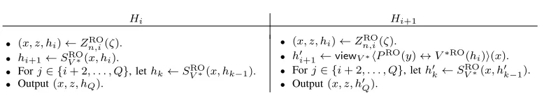
UsingZn,i, rewrite the Hi andHi+1 hybrids, as shown

in Table 1. Since we assumed that Dn can distinguish the hybrids Hi and Hi+1 with non-negligible advantage

Ψ

Q, there exists an advice ζ, a poly-size circuit Zn,i and a poly-size distinguisher D_n0 which—using the oracle-dependent auxiliary input generated by Zn,i on ζ (i.e.

hi)— distinguishes betweenhi+1 andh0i+1 with the same

advantage: Just simulateSV∗ forQ−i−1rounds (as above)

to obtain either hQ orh0Q, and then output asDn does. Now we exploit theK whose existence is guaranteed by Definition 13:KD0_n,RO_{runs in (expected) time}_poly(_Q₍_n₎_, Ψ−1₎_{, and generates an output so that} _D0

n can merely distinguish between hybridsHi andHi+1 with negligible

probability. Along the same line of reasoning, if a poly-size circuit D_n00 distinguishes between any two adjacent hybrids,KDn00,RO _{can fill the distinguishing gap. Therefore,}

all hybrids H_i0 and H_i0₊₁ (generated by K instead of

SV∗) are computationally indistinguishable. We conclude

that the extreme hybrids H0

0 andHn0 are computationally indistinguishable, and the theorem follows.

5.3 A New Protocol

It is easy to show that Protocol 1 is not ZK under Definition 13. An informal proof follows: LetZn compute

x ← SAMP(descfn) and y ← EVAL(descfn, x), and output z = y || RO(RO(x)). A cheating verifier V∗

forwardsyto the prover (or simulator), instead of computing it as prescribed. On receiving the response from the honest prover (which should bew= RO(x)by definition),V∗just queries RO at w, and accepts if RO(w) = RO(RO(x)). (The right-hand side is extracted fromz). On the other hand, to compute x, the simulator must either inverty or invert

RO; yet both tasks are infeasible for it. Letw_bbe the output of the simulator. To check the output, the distinguisherDn simply queriesROat w_b, and compares the answer to the second component inz (i.e.RO(RO(x)). Note that in this case,Dn does notknowthe value ofx, so its queries does not help any extractorK.

To fix this problem, we propose Protocol 3, which exploits Pass’ commitments [38]: To commit to a stringx

in the ROM, choose a randoms, and send(s,RO(x||s)).

Note that there is no decommitment phase, since the prescribed verifier already knowsx.

PROTOCOL3:

• Common Input: Description of fn. • Prover’s Auxiliary Input: tn. • Protocol Description:

1) V computesx←SAMP(desc(fn))and

y←EVAL(desc(fn), x), and sendsy toP. 2) The efficientproverP computes

x←INV(desc(fn), tn, y), chooses s←R{0,1}|x|, computes w←RO(x||s), and sends(s, w)toV. • Verification:V accepts ifw= RO(x||s), and rejects

otherwise.

Theorem 6. Assuming thatF ={fn} is a collection of trapdoor one-way permutations, Protocol 3 possesses the following properties:

(i) It is ZK under Definition 13. (ii) It is not EPRO ZK.

Proof: Each statement is proven separately:

(i) Let Z ={Zn} be as in Definition 13. On common and auxiliary inputs(desc(fn), ζ), letZnRO output the stringz. This string might include, among other things, a list ` = {(qi, ai)} of queries qi to the RO, along with the corresponding answerai= RO(qi).12 We call a query fresh if it does not belong to `. Note that z

(and in particular,`) might be encoded in such a way that it can be understood only by Z,V∗, andD, but it is incomprehensible by SV∗ or K.

On input (desc(fn), z), the simulator first obtainsy fromV∗. It then computesx0 ←SAMP(desc(fn)), and

s0 ←R{0,1}|x

0_|

. It then computes w0←RO(x0||s0), and outputs (desc(fn), y, s0, w0, r, z). (Here,r denotes the random tape of V∗.)

If the list` containsT queries (which is a polynomial in n since Zn is a poly-size circuit), the probability that x0||s0 is a fresh query is1− T

22|x|, which is an

overwhelming quantity assuming that |x| is super-logarithmic in n. This is indeed the case, because otherwise it would be easy to invert fn for alln. Now, if the queryx0_||_s0 _{is actually fresh, the} oracle-dependent auxiliary input does not help Dn to distin-guish the real and simulated view without first making

12. Anaimight be a function applied to several other answers. However,

(13)

query toRO. In this case, we can prove—similar to the proof of Lemma 2—that if Dn distinguishes the two distributions, there exists a knowledge extractorK

which can output xby monitoring the queries of Dn. However, if the query x0 || s0 is not fresh, Dn can distinguish the two distributions without making any queries toRO. In this case,Kmay resort to exhaustive search, which is justifiable because the probability of

SV∗ query not being fresh is negligible. Alternatively,

K might test any T+ 1 new queries, among which one will be certainly fresh (the size ofz can be used to obtain an upper bound for the value of T). (ii) To be EPRO ZK, the simulator should output a list

L at which RO is programmed. It must also output a pair (r,RO[L](x||r)), where RO[L] denotesRO

programmed according to the pairs inL.

There are two possible ways for the simulated view to be accepted:

a) The listLincludes the queryx||r. The probability of this event happening for infinitely manyn’s is negligible, because it meansSV∗ managed to invert

fn(y)and obtainx.

b) Ldoes not include the queryx||r, but the simulator manages to query RO at point x|| r. Again, this happens with negligible probability for infinitely many n’s, since otherwise we could exhibit an inverter forF (see Lemma 1 for a similar proof). Therefore, Protocol 3 is not EPRO ZK.

6 C

ONCLUSIONS AND

F

UTURE

W

ORK

This paper started by describing the notion of approxima-bility, an important concept in defining many cryptographic primitives such as pseudorandom generators and zero-knowledge protocols. Then, two hierarchies of successive weakenings of approximability were constructed, and it was shown that the some levels of the hierarchy can be separated relative to a random oracle (RO). Based on the semi-strong notion ofK-approximability, we described a zero-knowledge protocol, and proved the sequential composition theorem for a modified version of this protocol.

We believe that the most important task is to remove the need for the RO, and replace it with some suitable assumption. One possible solution is to extract the re-quired properties which the RO satisfies, and try to find a cryptographic primitive which satisfies these constraints (similar to [39], [40], [41]). Specifically, we believe that a suitable assumption, similar to the knowledge-of-exponent assumption (KEA) [42], [43], [44], [41] may prove useful. We are currently studying the plausibility of the following assumption (stated intuitively): For any PPTM D which distinguishes with non-negligible advantage between(fn(x),

gr, grx, z)and(fn(x), gr, gs, z), wherepandq= (p−1)/2 are primes, g∈Z∗p has orderq, andr andsare uniformly selected from Zq, there exists another PPTM S which outputs x. This assumption can be seen as a decisional

version of the KEA, and can be used to provide a weak

uniform ZKprotocol based on Protocol 3, in the standard model.

It is also interesting to study the closedness of the new definitions under other types of compositions. Moreover, separating various levels of the two hierarchies from each other is desirable.

R

EFERENCES

[1] S. Goldwasser and S. Micali, “Probabilistic Encryption & How to Play Mental Poker Keeping Secret All Partial Information,” inProceedings of the 14th Annual ACM Symposium on Theory of Csomputing(STOC ’82), (New York, NY, USA), pp. 365–377, 1982. See [4] for the

journal version.

[2] A. C.-C. Yao, “Theory and Applications of Trapdoor Functions (extended abstract),” in Proceedings of the 23rd Annual IEEE Symposium on Foundations of Computer Science(FOCS ’82), pp. 80– 91, IEEE, 1982.

[3] M. Blum and S. Micali, “How to Generate Cryptographically Strong Sequences of Pseudo-Random Bits,” in Proceedings of the 23rd Annual IEEE Symposium on Foundations of Computer Science(FOCS ’82), (Washington, DC, USA), pp. 112–117, IEEE Computer Society,

1982. See [5] for the journal version.

[4] S. Goldwasser and S. Micali, “Probabilistic Encryption,”Journal of Computer and System Sciences(JCSS), vol. 28, no. 2, pp. 270–299, 1984. See [1] for the conference version.

[5] M. Blum and S. Micali, “How to Generate Cryptographically Strong Sequences of Pseudo-Random Bits,”SIAM Journal on Computing, vol. 13, pp. 850–864, November 1984. See [3] for the conference version.

[6] S. Goldwasser, S. Micali, and C. Rackoff, “The Knowledge Complex-ity of Interactive Proof Systems,” inProceedings of the 17th Annual ACM Symposium on Theory of Computing, pp. 291–304, 1985. [7] S. Goldwasser, S. Micali, and C. Rackoff, “The Knowledge

Com-plexity of Interactive Proof Systems,”SIAM Journal on Computing, vol. 18, no. 1, pp. 186–208, 1989.

[8] O. Goldreich and Y. Oren, “Definitions and Properties of Zero-Knowledge Proof Systems,”Journal of Cryptology, vol. 7, pp. 1–32, 1994. See [45] for the conference version.

[9] O. Goldreich and H. Krawczyk, “On the Composition of Zero-Knowledge Proof Systems,”SIAM Journal on Computing, vol. 25, no. 1, pp. 169–192, 1996. See [46] for the conference version. [10] G. Brassard, D. Chaum, and C. Cr´epeau, “Minimum Disclosure

Proofs of Knowledge,”Journal of Computer and System Sciences

(JCSS), vol. 37, no. 2, pp. 156–189, 1988.

[11] B. Barak, “How to Go Beyond the Black-Box Simulation Barrier,” in

Proceedings of the 42nd Annual IEEE Symposium on Foundations of Computer Science(FOCS ’01), (Las Vegas, Nevada, USA), pp. 106– 115, IEEE Computer Society, 2001.

[12] C. Dwork and L. Stockmeyer, “2-Round Zero Knowledge and Proof Auditors,” inProceedings of the 34th Annual ACM Symposium on Theory of Computing (STOC ’02), (Montr´eal, Quebec, Canada), pp. 322–331, ACM, 2002.

[13] R. Pass, “Simulation in Quasi-Polynomial Time, and Its Application to Protocol Composition,” inAdvances in Cryptology—EUROCRYPT 2003, vol. 2656 ofLecture Notes in Computer Science, pp. 642–643, Springer Berlin / Heidelberg, 2003.

[14] E. Birrell and S. Vadhan, “Composition of Zero-Knowledge Proofs with Efficient Provers,” in Theory of Cryptography—TCC ’10, vol. 5978 of Lecture Notes in Computer Science, pp. 572–587, Springer Berlin / Heidelberg, 2010. Full version is available at http://eprint.iacr.org/2009/604.

[15] C. Dwork, M. Naor, O. Reingold, and L. J. Stockmeyer, “Magic Functions,” inProceedings of the 40th Annual IEEE Symposium on Foundations of Computer Science(FOCS ’99), (New York, NY, USA), pp. 523–534, IEEE Computer Society, 1999. See [20] for the full version.

[16] O. Goldreich,Computational Complexity: A Conceptual Perspective. New York, NY, USA: Cambridge University Press, 1 ed., 2008. [17] M. S. Dousti, “Beating Nonuniformity by Oracle Access.” Online