INFLUENCE OF MOTION ON THE EDGE-DIFFRACTION
M. Idemen
Department of Mathematics Yeditepe University
34755 Kayisdagi, Erenkoy, Istanbul, Turkey
A. Alkumru
Department of Electronics Engineering Gebze Institute of Technology
41400, Gebze, Kocaeli, Turkey
Abstract—The aim of the present paper is to reveal the effect of motion on the scattering by an edge. To this end one considers a canonical structure formed by a perfectly conducting half-plane illuminated by a time-harmonic and uniformly moving infinitely long line source. The relevant line source is located parallel to the edge and moves with a constant velocity which is also parallel to the half-plane. This is the dual of a previously studied problem in which the half-plane was moving uniformly. The present problem is first reduced into a Wiener-Hopf problem in thesense of distributionand then solved by an ad-hoc method. The edge-diffracted field is discussed in detail.
1. INTRODUCTION
modern swift vehicles and mobile antennas can be enumerated among simple examples.
An exact analysis for the case where the motion is accelerated can only be formulated in the framework of the General Theory of Relativity, which causes rather tough and complicated mathematical difficulties. Therefore, the works devoted to this kind of problems are very few in the open literature. However, when the motion is uniform, an exact analysis can sometimes be done with simple mathematical tools by using the concepts of the Special Theory of Relativity. So, in the open literature, there are many interesting works devoted to the case of uniformly moving scatterers. Among them one can enumerate, for example those which concern moving half-spaces or planes [1– 5], cylinders [5–10], strips [11, 12], wedges [13–15], half-planes and edges [16] and bodies of arbitrary shapes [5, 17–24]. A recent analysis performed in [16], which considers the scattering of a plane wave by a uniformly moving half-plane reveals the effect of the motion on the reflection, refraction, aberration, frequency shift, etc. The planar structure of the incident wave considered in [16] permitted one to reduce the problem into the solution of Helmholtz equation which is much more simple as compared to the time-depending wave equation. If the wave is not planar, it is not possible to benefice of the advantages provided by the complex representation of the monochromatic waves. In such a case it seems better to assume that it is the source which is in motion. As far as we know, the investigations devoted to this case also is very few in the available literature. [25, 26] can be cited as significant examples on this subject.
The aim of the present paper is the investigation of the effect of motion on the edge diffraction of a cylindrical wave. To this end one considers the canonical structure formed by a perfectly conducting half-plane illuminated by a uniformly moving infinitely long line source. One assumes that the line source is located parallel to the edge of the half-plane and moves in a direction which is parallel to the half-plane. In what follows, in Section 2 one formulates the problem in its most general form. In Sections 3 and 4 one considers the solution of the problem and analysis of the excited fields, respectively. Finally, in Section 5 one presents an illustrative example to see the variation of the edge-diffracted wave with respect to normalized time.
2. FORMULATION OF THE PROBLEM
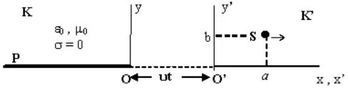
of a perfectly conducting sheet. In Kan infinitely long line source S ≡ {x = a, y = b, z ∈ (−∞,∞)} emits a cylindrical wave of ω. In the problem to be addressed in this work the line source S (and K) makes a uniform rectilinearmotion in vacuum with respect to the half-plane P (and K) (see Fig. 1). Then the problem consists of the investigation of the scattered wave to be observed inK. To this end we first use the well-known Lorentz transformation formulas to transform the expressions of the charge and current densities given inK intoK, and then consider and solve the problem in K.
Figure 1. A source moving with velocity υ =υex.
Let the clocks in K and K are so adjusted that O ≡ O when t = t = 0. Here t and t show the times measured in K and K, respectively. We assume that the incident wave is generated by the current and charge densities given as follows:
ρ = 0, (1a)
J = Icos(ωt−ϕ)δ(x−a)δ(y−b)ez. (1b)
Here ez shows the unit co-ordinate vector in the direction of Oz
-axis whileδ(.) is the usual Dirac distribution. In accordance with the Special Theory of Relativity one writes then (see [27] or [28])
x =γ(x−vt), y =y, z=z, t =γ(t−vx/c2) (2)
J =J−[1−γ](J·v)v
v2 +γρv (3a)
and
ρ=γ(ρ+J·v/c2). (3b) Here γ stands for
γ = 1
1−v2/c2. (4)
From (1a)–(3b) one gets
ρ = 0, (5a)
In the expressions given aboveex is the unit co-ordinate vector parallel
toOx-axis,v=vex is the velocity of the sourceS, c is the velocity of
the wave in the free-space whileω denotes
ω=γω. (5c)
From the expressions of the source densities given by (5a), (5b) one concludes that the electric fields of both the incident and the scattered waves are parallel to the edge. If the total electric field is written as
E(x, y, t) =u(x, y, t)ez, (6)
then the function u(x, y, t) satisfies the non-homogeneous wave equation
∆u− 1 c2
∂2u ∂t2 = µ
∂(J·ez)
∂t
= −µI[ωsin(ωt−ωvx/c2−ϕ)δ(xγ−a−γvt)
+γvcos(ωt−ωvx/c2−ϕ)δ(xγ−a−γvt)]δ(y−b) (7a)
in the sense of distribution outside the half-plane P under the continuity, boundary and radiation conditions given as follows:
u(x,+0, t) = u(x,−0, t); x, t∈(−∞,∞) (7b) ∂
∂yu(x,+0, t) = ∂
∂yu(x,−0, t); x >0, t∈(−∞,∞) (7c) u(x,+0, t) = u(x,−0, t) = 0; x <0, t∈(−∞,∞) (7d) u(x, y, t)∼outgoing wave forr =
x2+y2 → ∞, t∈(−∞,∞). (7e)
In (7a) δ denotes the derivative of delta Dirac function with respect to its argument.
3. SOLUTION OF THE PROBLEM
Let the double Fourier transform of the functionu(x, y, t) with respect tox andt, say ˆu(α, y, β), be defined via
ˆ
u(α, y, β) =
∞
x=−∞ ∞
t=−∞
The inverse transform is then
u(x, y, t) = 1 (2π)2
∞
β=−∞
L
ˆ
u(α, y, β)e−iαxe−iβtdαdβ. (8b)
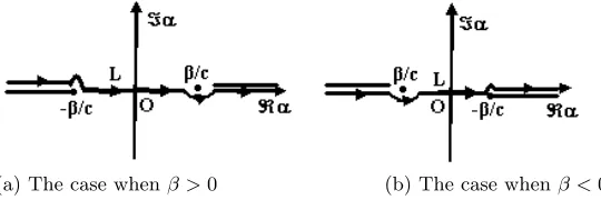
Here L denotes the real axis indented above (−β/c) and below (β/c) as shown in Fig. 2.
(a) The case whenβ >0 (b) The case whenβ <0 Figure 2. The integration line L in the complexα-plane.
The application of the double transformation (8a) to (7a) yields
d2uˆ dy2 −λ
2(α, β)ˆu=K(α, β)δ(y−b), β ∈(−∞,∞), α∈L, (9)
whereλ(α, β) stands for the square-root function λ(α, β) =
α2−β2/c2 (10)
defined in the complex α-plane cut as shown in Fig. 2 with the condition λ(0, β) =−iβ/c whileK(α, β) is given by
K(α, β) = iπµI γ e
iαa/γ
ω
γ2 +αv
e−i
ωva γc2+ϕ δ
β+ ω γ2 +αv
−
ω γ2 −αv
ei
ωva γc2+ϕ δ
β− ω γ2 +αv
. (11) The solution of (9), which satisfies the radiation condition (7e) is given by
ˆ
u(α, y, β) =
A(α, β)e−λ(α,β)y ; y > b B(α, β)e−λ(α,β)y+C(α, β)eλ(α,β)y ; 0< y < b
D(α, β)eλ(α,β)y ; y <0.
The expressions of the coefficients A(α, β), B(α, β), C(α, β) and D(α, β) can be obtained through the relations required by (9) and (7b)–(7d), which yield
A(α, β)e−λ(α,β)b−B(α, β)e−λ(α,β)b−C(α, β)eλ(α,β)b = 0 (13a) A(α, β)e−λ(α,β)b−B(α, β)e−λ(α,β)b+C(α, β)eλ(α,β)b=−K(α, β)
λ(α, β) (13b)
B(α, β) +C(α, β)−D(α, β) = 0 (13c)
D(α, β) = Φ+(α, β) (13d)
B(α, β)−C(α, β) +D(α, β) =−Φ−(α, β)
λ(α, β) . (13e) The functions Φ+(α, β) and Φ−(α, β) appearing in (13d)–(13e) are yet unknown and defined by
Φ+(α, β) =
∞
0
∞
−∞
u(x,0, t)eiβtdt
eiαxdx (14a)
and
Φ−(α, β) =
0
−∞
∞
−∞
∂
∂yu(x,+0, t)− ∂
∂yu(x,−0, t)
eiβtdt
eiαxdx. (14b) From (14a)–(14b) it is obvious that the functions Φ+(α, β) and
Φ−(α, β) are regular in the upper half-planeα >0 and in the lower half-plane α < 0, respectively. Moreover, since u(x,0, t) = O(1) when x →+0 while ∂y∂u(x,±0, t) =O(x−1/2) whenx → −0 [29], the functions Φ±(α, β) have also the following asymptotic behaviors when α→ ∞ [30]:
Φ+(α, β) = O(1/α) as α→ ∞ inα >0 (15a) Φ−(α, β) = O(α−1/2) as α→ ∞ inα <0. (15b) From (13a)–(13b) one gets
C(α, β) =−K(α, β) 2λ(α, β)e
−λ(α,β)b (16a)
and
A(α, β) =B(α, β)− K(α, β) 2λ(α, β)e
This shows that the coefficient C(α, β) is known beforehand and A(α, β) is obtained in terms of B(α, β) which can be expressed by the use of (13c)–(13e) as
B(α, β) = Φ+(α, β) + K(α, β) 2λ(α, β)e
−λ(α,β)b (17a)
and
B(α, β) =−Φ+(α, β)−Φ
−(α, β)
λ(α, β) −
K(α, β) 2λ(α, β)e
−λ(α,β)b. (17b)
To determine Φ+(α, β) and Φ−(α, β) appearing in (17a)–(17b) one has to eliminate B(α, β) through these equations. Thus, one gets a functional equation of the Wiener-Hopf type satisfied by Φ+(α, β) and Φ−(α, β), namely:
Φ−(α, β) λ(α, β) + 2Φ
+(α, β) =−K(α, β)
λ(α, β)e
−λ(α,β)b, α ∈L. (18)
By substituting the expression ofλ(α, β) andK(α, β) given by (10) and (11) into (18) and multiplying both sides of this equation byα+β/c one gets
Φ−(α, β)
α−β/c + 2Φ
+(α, β)α+β/c=f
1(β)δ(α−β1) +f2(β)δ(α−β2)
(19) whereβ1 and β2 are given by
β1 = −
1
v(β+ω/γ
2), (20a)
β2 = −
1
v(β−ω/γ
2). (20b)
In (19) the functions f1(β) and f2(β) refer to
f1(β) =
iπµI γ|v|e
−i
ωva
γc2+ϕ βe−
λ1(β)beiaβ1/γ
β1−β/c
(21a)
and
f2(β) =
iπµI γ|v|e
i
ωva
γc2+ϕ βe−λ2(β)beiaβ2/γ
β2−β/c
(21b)
with
λ1(β) =λ(β1, β) =
β
v + ω vγ2
2
−β2
and
λ2(β) =λ(β2, β) =
β
v − ω vγ2
2
−β2
c2. (22b)
Here it is worthwhile to remark that in order to obtain the expressions given by (20a), (20b) and (21a), (21b), the following identities related to Dirac distribution have also been considered:
δ(vα+ζ) = 1 |v|δ
α+ζ v
, (23a)
f(α)δ(α−ζ) = f(ζ)δ(α−ζ). (23b) It is obvious that the expression given by (19) constitutes a Wiener-Hopf equation which involves Dirac distributions. To solve this kind of an equation with respect to the parameterα one can use the well-known Plemelj-Sokhotski formulas [31] which yields
δ(α) = 1 2πi
1 α−i0 −
1 α+i0
= 1 2πiεlim→+0
1 α−iε −
1 α+iε
. (24) With the use of (24), the functional equation (19) can be rewritten as
Φ−(α, β)
α−β/c + 2Φ
+(α, β)α+β/c=f+(α) +f−(α), (25a)
where the functionsf+(α) andf−(α) which are regular in the upper half-plane α > 0 and in the lower half-plane α < 0, respectively, are defined by
f+(α) =− 1 2πiεlim→+0
f1(β)
α−β1+iε
+ f2(β) α−β2+iε
(25b)
and
f−(α) = 1 2πiεlim→+0
f1(β)
α−β1−iε
+ f2(β) α−β2−iε
. (25c) Thus functions Φ+(α, β) and Φ−(α, β) are determined immediately through the classical Wiener-Hopf technique [30], namely:
Φ+(α, β) = i 4πα+β/c
f1(β)
α−β1+i0
+ f2(β) α−β2+i0
(26a)
and
Φ−(α, β) =
α−β/c 2πi
f
1(β)
α−β1−i0
+ f2(β) α−β2−i0
. (26b)
4. ANALYSIS OF THE FIELD
By inserting first the expressions for the coefficients A(α, β), B(α, β), C(α, β) andD(α, β), which were obtained in the previous section, into (12) and then considering (8b) one obtains the expression of the total field in the whole space. In what follows we will consider the regions y > b,y∈(0, b) andy <0 separately.
4.1. Waves in the Region y > b
By inserting (16b), (17a) and (12) in (8b) one gets the total field in the regiony > b as follows:
u(x, y, t) =uinc(x, y, t) +uref(x, y, t) +us(x, y, t). (27a) Here we put
uinc(x, y, t) = − 1 8π2 ∞ β=−∞ L K(α, β) λ(α, β)e
−λ(α,β)(y−b)−iαx−iβtdαdβ(27b)
uref(x, y, t) = 1 8π2 ∞ β=−∞ L K(α, β) λ(α, β)e
−λ(α,β)(y+b)−iαx−iβtdαdβ (27c)
and
us(x, y, t) = 1 4π2 ∞ β=−∞ L
Φ+(α, β)e−λ(α,β)y−iαx−iβtdαdβ. (27d)
If one inserts the expression ofK(α, β) given by (11) into the integrand of (27b) and evaluates the resulting integral onL, then one gets
uinc(x, y, t) = iµI 8πγ|v|e
−i
ωva γc2+ϕ
∞
β=−∞
βe−λ1(β)(y−b)+i
β v+
ω
vγ2 x−
a γ
−iβt
λ1(β)
dβ
+ iµI 8πγ|v|e
i
ωva γc2+ϕ
∞
β=−∞
βe−λ2(β)(y−b)+i
β v−
ω
vγ2 x−
a γ
−iβt
λ2(β)
dβ.
(28)
the half-planeP. Therefore it is the wave emitted by the moving line source i.e., “the incident wave”.
By repeating the same procedure which transformed (27b) to (28) foruref(x, y, t) given by (27c) one obtains also
uref(x, y, t) =− iµI 8πγ|v|e
−i
ωva γc2+ϕ
∞
β=−∞
βe−λ1(β)(y+b)+i
β v+
ω vγ2 x−
a γ
−iβt
λ1(β)
dβ
− iµI 8πγ|v|e
i
ωva γc2+ϕ
∞
β=−∞
βe−λ2(β)(y+b)+i
β v−
ω
vγ2 x−
a γ
−iβt
λ2(β)
dβ. (29)
A comparison of (29) with (28) shows that uref(x, y, t) is obtained from uinc(x, y, t) by making the substitution I → −I and b → −b in
(28). Therefore uref(x, y, t) can be interpreted as the field which is
created by the image source. In other words, uref(x, y, t) consists of the wave reflected from the conducting plane P. It is also important to emphasize that in some region of the space this reflected wave will be cancelled by a pole contribution which will appear during the evaluation of the integral in (27d).
As to the last term in (27a), from (27d) and (26a) one writes it as
us(x, y, t) = i 16π3 ∞ β=−∞ L f 1(β)
α−β1+i0
+ f2(β) α−β2+i0
e−λy−iαx−iβt
α+β/c dαdβ. (30) To recast the latter into more propitious form, we make the substitutions
α=−β
c cosτ, λ(α, β) =−i β
c sinτ, dα= β
c sinτ dτ (31a) and
x=Rcosφ, y=Rsinφ; R=
x2+y2, φ∈(0, π) (31b)
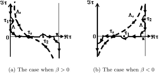
which map the integration line L onto Λ shown in Fig. 3. Thus we have
us(x, y, t) = √ c 16iπ3 ∞ β=−∞
(a) The case whenβ >0 (b) The case whenβ <0
Figure 3. The integration line Λ and the steepest descent line Λs in
the complexτ-plane.
×
Λ
sinτ eiβcRcos(τ−φ)
(cosτ + ˜β1)
√
1−cosτdτ
dβ
+ √
c 16iπ3
∞
β=−∞
β−1/2f2(β)e−iβt
×
Λ
sinτ eiβcRcos(τ−φ)
(cosτ + ˜β2)
√
1−cosτdτ
dβ (32a)
with
˜ β1 =
c
ββ1, β˜2= c
ββ2. (32b)
Now let us use the Cauchy theorem and translate Λ onto the steepest-descent line Λs which passes through the saddle pointτs =φ. When
β > 0, one has τs = φ < τ2 = arccos(−β˜2) and crosses the pole at
τ2 = arccos(−β˜2) in translating Λ onto Λs (see Fig. 3(a)). Conversely,
when β < 0, one has τs = φ < τ1 = arccos(−β˜1) and the pole at
τ1 = arccos(−β˜1) is crossed in translating Λ onto Λs (see Fig. 3(b))
when τs=φ > τ1 = arccos(−β˜1) (see Fig. 3(b)). Thus, by taking also
into account the contributions which will come from the poles, (32a) can be rearranged as follows:
up(x, y, t) = 1 8π2 ∞ β=−∞
f1(β)
e−λ1(β)y−iβ1x−iβt
β1+β/c
+f2(β)
e−λ2(β)y−iβ2x−iβt
β2+β/c
dβ(34a)
and
ud(x, y, t) = √ c 16iπ3 ∞ β=−∞
β−1/2f1(β)e−iβt
Λs
sinτ eiβcRcos(τ−φ)
(cosτ + ˜β1)
√
1−cosτdτ
dβ + √ c 16iπ3 ∞ β=−∞
β−1/2f2(β)e−iβt
Λs
sinτ eiβcRcos(τ−φ)
(cosτ+ ˜β2)
√
1−cosτdτ
dβ. (34b)
up(x, y, t) consists of the pole contributions. By using (21a), (21b) in (34a) one can easily show that
up(x, y, t) =−uref(x, y, t) (35) in the region defined byτ1< φ < τ2.
As to the last term ud(x, y, t) in (33), it gives the edge-excited diffracted wave. The integrals in (34b), written on Λs and β ∈
(−∞,∞) , can be evaluated asymptotically by saddle-point technique [30] for points far away from the edge. The saddle points connected with the parametersτ andβ are
τs=φ (36)
and
βs=ω
1− v c
χ(x, y, t)
b2/γ2+χ2(x, y, t)
, (37)
respectively. Here χ(x, y, t) is given by
χ(x, y, t) =v(t−R/c) +a/γ. (38) Thus we get finally
ud(x, y, t) ∼ µIb √
c2−vc
4γ√π
sinφ √
1−cosφ 1 √
R
[b2/γ2+χ2]−1/2
×
b2/γ2+χ2−(v/c)χ
(v/c−cosφ)b2/γ2+χ2−(1−cosφv/c)χ
× F
kβ 2
2ω R
φ−arccos(c/v−cω/β2γ2) 2
×ei
3π/4+ϕ+ωR/c+ω√b2/γ2+χ2/c−ωt!
, (39a)
where F(η) is the following function which can be expressed through the classical error function [32]:
F(η) =√ηe−iηerf c
e−iπ/4√η . (39b) 4.2. Waves in the Region 0< y < b
By replacing first C(α) and B(α) in (12) by their expressions given by (16a) and (17a) and then inserting the result into (8b) one gets the expression of the field in the region 0 < y < b. A scrutinization shows that the terms are identical to the terms obtained in the previous Section 4.1. Therefore the wave in the region y∈(0, b) consists of the analytical continuation of that in y > b.
4.3. Waves in the Region y <0
By considering (13d) and (26a) in (12), the total field in the region can be written from (8b) as follow:
u(x, y, t) = i 16π3
∞
β=−∞
L
f1(β)
α−β1+i0
+ f2(β) α−β2+i0
eλy−iαx−βt
α+β/cdαdβ. (40) By making the same substitutions given by (31a), (31b) forφ∈(−π,0) and following the same procedure, as explained in the Section 4.1., on the stage of translation the integration line Λ onto the steepest-descent line Λs which passes through the saddle pointτs=−φ, the field given
by (40) can be rearranged as
us(x, y, t) =up(x, y, t) +ud(x, y, t) (41) whereup(x, y, t) is the expression of the field which is obtained from the residue contribution of the polesτ1 and τ2. The computation of these
pole contributions shows that up(x, y, t) is identical with the incident
field ui(x, y, t) in the lit region defined by −τ
2 < φ < −τ1. In (41)
5. AN ILLUSTRATIVE EXAMPLE
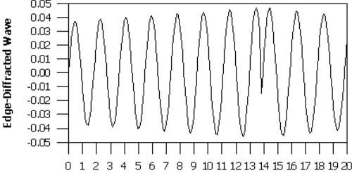
In order to give an idea about the variation of the edge-diffracted wave with respect to time normalized by (˜λ/c), one computes the expression of ud(x, y, t) given by (37a) at the point Q(−λ,˜ 10˜λ,0) for v = 2c/3, I = 10 mA and a=b= 100˜λ. Here ˜λ and c stands for the wave-length of the monochromatic wave. Fig. 4. given below shows this variation in the time intervalt∈(0,20˜λ/c).
Figure 4. Variation of the edge diffracted wave with normalized time.
From this figure it is obvious to remark that the edge-excited wave has always the same oscillation whenever the source is approaching the observation point or going far away from it. The non-periodic variation of the wave is also observed.
ACKNOWLEDGMENT
This work was supported by TUBA (Turkish Academy of Sciences).
REFERENCES
1. Pauli, W.,Theory of Relativity, Pergamon Press, New York, 1958. 2. Yeh, C., “Reflection and transmission of electromagnetic waves by moving dielectric medium,”J. of Appl. Phys., Vol. 36, 3513–3517, 1965.
3. Lee, S. W. and Y. T. Lo, “Reflection and transmission of electromagnetic waves by moving uniaxially anisotropic medium,”
J. of Appl. Phys., Vol. 8, 870–875, 1967.
5. Censor, D., “Broadband spatiotemporal differential-operator representations for velocity depending scattering,” Progress In Electromagnetics Research, PIER 58, 51–70, 2006.
6. Lee, S. W. and R. Mittra, “Scattering of electromagnetic waves by a moving cylinder in free space,” Canadian J. of Phys., Vol. 45, 2999–3007, 1967.
7. Censor, D., “Scattering of electromagnetic waves by a cylinder moving along its axis,”Microwave Theory and Techn., Vol. MTT-17, 154–158, 1969.
8. De Zutter, D. and J. Van Bladel, “Scattering by cylinders in translational motion,” IEE Microwaves, Optics and Antennas, Vol. 1, 192–196, 1977.
9. Borghi, R., F. Gori, M. Santersiero, F. Frezza, and G. Schettini, “Plane wave scattering by conducting cylindernear a plane surface: A cylindrical wave approach,”J. Optical Soc. Amer. - A, Vol. 13, 483–493, 1996.
10. Idemen, M. and A. Alkumru, “Influence of the velocity on the energy patterns of moving scatterers,”J. of Electromagn. Waves and Appl., Vol. 18, 3–22, 2004.
11. Tsandoulas, G. N., “Low-frequency diffraction by mowing conducting strips,”J. Opt. Soc. Amer., Vol. 59, 1357–1360, 1969. 12. Hunter, J. D., “High-frequency diffraction by a moving conducting strip,” IEEE Trans. Antennas and Propagat., Vol. 20, 792–794, 1972.
13. Lang, K. C., “Diffraction of electromagnetic waves by a moving impedance wedge,” Radio Sci., Vol. 6, 655–663, 1971.
14. De Cupis, P., P. Burghignoli, G. Gerosa, and M. Marziale, “Electromagnetic wave scattering by a perfectly conducting wedge in uniform translational motion,” J. of Electromagn. Waves and Appl., Vol. 16, 345–364, 2002.
15. Tsandoulas, G. N., “Electromagnetic diffraction by a moving wedge,”Radio Sci., Vol. 3, 887–893, 1968.
16. Idemen, M. and A. Alkumru, “Relativistic scattering of a plane-wave by a uniformly moving half-plane,” IEEE Trans. Antennas and Propagat., Vol. 54, 3429–3440, 2006.
17. Ott, R. H. and G. Hufford, “Scattering by an arbitrarily shaped conductor in uniform motion relative to the source of an incident spherical wave,”Radio Sci., Vol. 3, 857–861, 1968.
18. Censor, D., “Scattering in velocity-dependent systems,” Radio Sci., Vol. 7, 331–337, 1972.
scattering by an object in relativistic translational motion,” J. of Electromagn. Waves and Appl., Vol. 14, 1037–1062, 2000. 20. Twerski, V., “Relativistic scattering of electromagnetic waves by
moving obstacles,”J. Math. Phys., Vol. 12, 2328–2341, 1971. 21. Censor, D., “Scattering by time-varying obstacles,” J. Sound
Vibration, Vol. 25, 101–110, 1972.
22. Michielsen, B. L., G. C. Herman, A. T. de Hoop, and D. De Zutter, “Three-dimensional relativistic scattering of electromagnetic waves by an object in uniform translation motion,”J. Math. Phys., Vol. 22, 2716–2722, 1981.
23. Tzikas, A. A., D. P. Chrissoulidis, and E. E. Kriezis, “Relativistic bistatic scattering by a uniformly moving random rough surface,”
IEEE Trans. Antennas and Propagat., Vol. AP-34, 1046–1052, 1986.
24. De Zutter, D., “Fourier analysis of the signal scattered by objects in translational motion, Part I and II,” Appl.Sci. Res., Vol. 36, 241–169, 1980.
25. Rabinovich, V. S. and I. Miranda, “Non uniformly moving source in electromagnetic waveguides,” Proceedings of Day on Diffraction, 193–202, 2003.
26. Shimura, T., H. Ochi, and Y. Watanabe, “Time-reversal communication with moving source-receiver in shallow water,”
Jap. J. Appl. Phys., Vol. 45, 4847–4852, 2006.
27. Moeller, C., The Theory of Relativity, 2nd edition, Oxford University Press, London, 1972.
28. Kong, J. A., Electromagnetic Wave Theory, John Wiley & Sons Inc., New York, 1990.
29. Idemen, M., Confluent Edge Conditions for the Electromagnetic Wave at the Edge of a Wedge Bounded by Material Sheets, Wave Motion, Vol. 2, No. 1, 37–55, 2000.
30. Noble, B., Methods Based on the Wiener-Hopf Techniques, Pergamon, Oxford, 1958.
31. Gel’fand, I. M. and G. E. Shilov,Les Distributions, Dunod, Paris, 1962.