The 3D structure of QCD and the roots of the Standard Model
P.J. Mulders1,a
1Nikhef Theory Group and Vrije Universiteit Amsterdam, De Boelelaan 1081, 1081 HV Amsterdam, the
Netherlands
Abstract. For many phenomenological applications involving hadrons in high energy
processes the hadronic structure can be taken care of by parton distribution functions (PDFs), in which only the collinear momenta of quarks and gluons are important. In prin-ciple the transverse structure, however, provides interesting new phenomenology. Taking into account transverse momenta of partons one works with transverse momentum depen-dent PDFs (TMDs), These allow all spin-spin correlations and also spin-orbit correlations that have a time reversal odd character and lead to new observables. In many theoretical developments the link to the collinear treatment is used. In this talk I will speculate on a novel view of the 3-dimensional (3D) structure of QCD, which fits in a broader study looking at the roots of the Standard Model of particle physics.
1 Introduction
In the abstract of this talk I emphasized the role of transverse components of the partonic momenta in parton distribution functions (PDFs), hence generalizing them to transverse momentum dependent (TMD) PDFs or in short TMDs. This extends upon the highly successful collinear description of high energy scattering processes where collinear PDFsf(x) only depending on the momentum fractionxin p=x P+. . .describe the partonic (quark and gluon) content of a proton with momentumP. One can think about jet physics, scale dependence, the role of Collins-Soper-Sterman (CSS) formalism to study transverse momenta in the perturbative regime [1], or soft collinear effective theories (SCET [2]). While collinear PDFs only can accomodate unpolarized and spin-spin correlations between hadron and partons, TMDs can accomodate spin-momentum correlations, important in accounting for single spin asymmetries and understanding azimuthal asymmetries in high energy scattering processes.
Most TMDs still have quite naturally the interpretation of momentum densities, now of the type f(x,p2
T), including the transverse component in p = x P+pT +. . ., which incorporate for instance
longitudinal-transverse spin correlations. One of the important issues in dealing with TMDs is that their operator structure necessarily involves (covariant) transverse derivatives, hence gluon fields. This leads for some of the TMDs, in particular the time reversal odd ones (important for single spin asymmetries) to process dependence and the occurrence of multiple functions, for instance for the socalled quark pretzelocity function and the linear gluon polarization. For these issues, I want to refer to contributions in the proceedings of DIS2015 [3] or QCD evolution 2015 [4] and references therein.
In this contribution I will focus on the question if there possibly could be more fundamental rea-sons for the success of collinear physics in QCD linked to the transition from 1D to 3D with the warning that the material in the next sections is very preliminary and at many points speculative [5]. I want to argue that the standard model and its particle content may naturally emerge in a world with anIO(1,1)⊗S U(3) spacetime-color symmetry broken down to a threefoldIO(1,3)⊗[S U(2)×U(1)] spacetime-electroweak symmetry for the asymptotic fields leaving only the electroweak charges for these asymptotic particle states. The bosonic excitations are the electroweak gauge bosons, the mass-less photon and massiveW andZ bosons, as well as the Higgs boson. Fermionic excitations come in three families of colorless (leptonic) excitations living inE(1,3) or they form three families of colored (quark) excitations living inE(1,1). Many features of the Standard Model emerge naturally. Taking a supersymmetric starting point solves the naturalness problem. There is an underlying left-right symmetry leading to custodial symmetry in the electroweak sector. In the spectrum one naturally has Dirac-type charged leptons and Majorana-type neutrinos. The electroweak behavior of the natu-rally confined quarks, accomodates fractional electric charges and the doublet and singlet structure of left- and right-handed quarks, respectively. Most prominent feature is the link between the number of colors, families and space directions.
2 A 1D supersymmetric starting point
As already indicated in the introduction, we take the 1D world serious as a starting point with operators H, P(combined into Pμor combined in the combinations P± = H±P) and the boost operator K generating the 2-dimensional Poincaré symmetry groupIO(1,1),
[H,P]=0, [K,H]=iPand [K,P]=iH, or [P+,P−]=0 and [K,P±]=±iP±, (1)
with Casimir operatorP2 = PμP
μ = H2−P2 = P+P−. The IO(1,1) symmetry can be combined with anS O(N) symmetry to obtain theIO(1,N) space-time symmetry. with as generatorsH,Pi,Ki andJ[i j](combined intoPμandJμν, of course after also including discrete space- and time-reversal symmetries.
Positive and negative energy (particle and anti-particle) eigenstates of the momentum operator have a space-time phase dependenceφk(x)=ei k·xwith (k0)2−k2=k−k+−k2T=M
2. These plane waves
are solutions of the Klein-Gordon equation (∂μ∂μ+M2)φ=0 or, with the appropriate Clifford algebra,
the Dirac equation (i/∂−M)ξ =0. For massless excitations in 1D one can distinguish independent right-movers, depending onx+, and left-movers, depending onx−. Expanded in these modes right-and left-hright-anded fields can be defined satisfying [P−, φR]=i∂+φR =0 and [P+, φL]=i∂−φL =0. For
massive fields left and right modes become coupled, while the other derivatives [P+, φR]=i∂−φRand
[P−, φL]=i∂+φLacquire roles as (front form) canonical momenta [6]. ForM =0 the fermion fields in
1D satisfyγ−ξR =γ+ξL =0 andξR/Lare independent good fields [7]. Massive fermion fields satisfy
the constraints
[P−, ξR]=i∂+ξR=−iMξL and [P+, ξL]=i∂−ξL=iMξR. (2)
As an additional ingredient, the Poincaré algebra can be extended to a supersymmetric algebra [8] with fermionic operatorsQR/L,
{QR,Q†R}=2P+=2P·n,¯ {QL,Q†L}=2P−=2P·n and {QR,QL}=0, (3)
[P±,QR/L]=0 and [K,QR/L]=±12i QR/L. (4)
The supersymmetry charges connect the fields,
The contact with the real world is made by considering the excitations of three real scalar and real fermionic (Majorana) fieldsφandξ, still in a single space dimension, however. If their masses are zero one can distinguish right-movers (R) and left-movers (L) as independent degrees of freedom, which for bosons is a simple doubling but for fermions coincides with right- and left-handed fermions. Including left-right coupling via a single massMand a single Yukawa coupling between the boson fields, linked in the supersymmetric situation to the coupling of fermions and bosons, we have basically the Wess-Zumino model [9] in two dimensions,
L = 1
2∂−φR∂+φR+ 1
2∂+φL∂−φL+ i
2ξR∂+ξR+ i
2ξL∂−ξL−V(φ, ξ)
= 1 2∂
μφ
S∂μφS +12∂μφP∂μφP+iψ/∂ψ−V(φ, ξ), (6)
where (real) right and left fields for bosons can be combined into (real) scalar (CP-even) and pseu-doscalar (CP-odd) fieldsφS/P = (φR ±φL)/
√
2. Real fermion fields can be combined in a (self-conjugate) spinorψ = (ξR,−iξL)/
√
2. Supersymmetry strongly restricts the interaction terms. The most compact expression is in terms of the scalar and pseudoscalar fields containing a mass term cou-pling left and right fields and a single Yukawa coucou-pling that also governs the fermion-boson coucou-pling,
V(φ, ξ) = 1
2(M+gφS) 2(φ2
S +φ2P)+12g 2φ2
P(φ2S +φ2P)+ψ(M+gφS +gφPγ1)ψ+λF (7)
usingγ5 =γ0γ1. The constraint is given by
λF = λ
4g
(M+2gφR
√
2)(M+2gφL
√
2)−M2=λg(gφS +M/2)2−g2φ2P−M2/4
. (8)
Defining M/2g ≡ v, we introduce fieldsφS +v ≡ vΦS andvΦP ≡ φP which can be re-defined as
ΦS = coshη andΦP = sinhη or if one likes one can use an imaginary representation for ΦP by
writingη=iθ. The bosonic part of the potential including constraint becomes
V(Φ) = v 2M2
2 Φ
2 SΦ2P =
v2M2
2 Φ
2
S(Φ2S −1) (9)
orV(Φ) = 18M2v2sinh2(2η). Defining|Φ|2 ≡ (Φ2
S + Φ2P)/2 = Φ2R + Φ2L we have|Φ|2 = cosh(2η)
and we have Φ2
S = |Φ|2 +1/2 and Φ2P = |Φ|2 −1/2. Looking at the minimum of the potential
(η=0 orθ=0) we see that the boson field acquires a vacuum expectation value which is right-left symmetric,ΦR = ΦL=|Φ|=1/
√
2 (orΦS =1 andΦP =0). The real excitations around the vacuum
are Majorana modesΨ = Ψc = (ξ,−iξ)/√2 and real scalar bosonic modesΦS/
√
2 = Φ = Φc = (1+H)/√2. Note thatφS = vH. The 1D pseudoscalar fieldφP can be identified as a vector field
writingi∂μΦR/L =(i∂μ±gAμ)φS/
√
2. In the ground stateAμ =0 and around the vacuum one has Aμ ≈ φP(nμ−n¯μ) or A+ = −A− ≈ φP. This suggests working with a complex fieldΦrather than
left and right fields that are CP symmetric,ΦR = Φ∗L. For a single field a globalU(1) symmetry is
not relevant and local symmetries don’t lead to dynamics either, but taking multiple scalar fields the symmetry pattern becomes much richer.
3 Symmetric extension to three fields
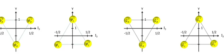
Figure 1.SU(3) quantum number assignments for bosonic (φ) and fermionic (ξ) excitations. The right-moving positively charged (φ+R,ξ+R) and neutral (φ0R,ξ
0
R) fields are in an isospin doublet withY = +1, while the
right-moving negatively charged (φ−R, ξR−) fields are in a weak isosinglet withY = −2. The left-moving negatively charged (φ−L,ξ−L) and neutral (φ0
L,ξ0L) fields are in an isospin doublet withY=−1 while the left-moving positively
charged (φ+L,ξ+L) fields are in a weak isosinglet withY = +2. The asymptotic fermion fields become the right-and left-hright-anded leptonic fields,ξR±/L→e±R/Landξ0R/L→ν
0 R/L.
inversion and time reversal symmetry, to extend thed =2 Poincaré symmetry to ad = 4 Poincaré symmetry. Implemented in Weyl mode, the asymptotic fields become real representations ofIO(1,3) living inE(1,3).
At this stage part of the freedom in fluctuations around the vacuum has been incorporated. The already accounted for realS O(3) rotations are identified with the subalgebra generated by theS U(3) generatorsλ2,−λ5andλ7, constituting the algebra of the factor group of the subgroupG=S U(2)× U(1) with generatorsλ1/2,λ2/2,λ3/2 andλ8/2. This subgroup contains theS U(3) Cartan subalgebra
consisting ofI3 = λ3/2 andY = λ8
√
3 that will serve as electroweak charge labels. Labelling the (massless) bosonic states using this Cartan subalgebra, gives fieldsφ[IR/3,LY](x,t) living inE(1,3). For two fields this would have been just aU(1) charge assigment after combining two real fields into complex fields. The basic recoupled bosonic and fermionic starting point for the three fields and their electroweak quantum numbers is illustrated in Fig. 1.
The fluctuations around the vacuum in space-time and internal space is also reflected in the co-variant derivative. We consider the possibilities
E(1,1) : iDμΦi=i∂μΦi+g a∈G
Aaμ(Ta)ijΦj, (10)
E(1,3) : iDμΦi=i∂μΦi+g a∈G
Aa
μ(Ta)ijΦj. (11)
The first expression for the covariant derivative applies to the fields inE(1,1) and accounts for local S U(3) gauge invariance. It involves eight (color) gauge fields also living in E(1,1). The second expression for the covariant derivative is relevant for (asymptotic) fields inE(1,3), coupling for the realcontinuousS O(3) transformations field and space rotations in such a way that there are no gauge fields for that part, and account for the complex fluctuations through four (electroweak) gauge fields living inE(1,3). Such a transition from 1D to 3D, in whatever way we implement it, does require that the Poincaré symmetry and internal symmetry are direct products [10].
To achieve this, we note that the embedding ofS O(3) directions intoS U(3) is not unique. The discrete symmetry groupA4 governs the possible oriented embeddings. For singlet representations
of the embedding group (A4) one can considerS U(3) ⊃S O(3)×A4×[S U(2)⊗U(1)]→ S O(3)⊗
embedding of the vacuum into theelectroweakembedding,
W†⎧⎪⎪⎪⎪⎪⎪⎪⎪ ⎪⎩
√ 1/3 √
1/3 √
1/3 ⎫⎪⎪⎪ ⎪⎪⎪⎪⎪ ⎪⎭= ⎧⎪⎪⎪ ⎪⎪⎪⎪⎪ ⎪⎩ 0 1 0 ⎫⎪⎪⎪ ⎪⎪⎪⎪⎪
⎪⎭ with W = 1 √ 3 ⎧⎪⎪⎪ ⎪⎪⎪⎪⎪ ⎪⎩
1 1 1
ω2 1 ω
ω 1 ω2
⎫⎪⎪⎪ ⎪⎪⎪⎪⎪
⎪⎭, (12)
whereω =exp(i2π/3). Since the starting point only hadS O(3) as a symmetry group, the vacuum indeed is not invariant underS U(2)⊗U(1) transformations, but it is neutral forQ=I3+Y/2. The
symmetry pattern and its breaking thus is summarized as
IO(1,1)⊗S U(3) ⊃ IO(1,1)×S O(3)
IO(1,3)
⊗S U(2)I⊗U(1)Y
→U(1)Q
.
All bosons and fermions, however, still do originate as (finite dimensional) representations of the basicS U(3) symmetry group, which will become important later. There are three families of particles corresponding to singlets ofA4. In 3D the interaction changes from a confining potential to a 1/r
(or Yukawa) potential between the (electroweak) charges, which thus can befree, in contrast to the (color)S U(3) charges that live in 1D.
4 Bosons and Fermions in the Standard Model
After the introduction of the covariant derivatives in Eqs 10 or 11, part of the potential is included in the term
DμΦ∗DμΦ = ∂μΦ∗∂μΦ + N CA 2 g
2AμA
μΦ∗Φ. (13)
WithCA(G =S U(3)) =4/3, the second term in Eq. 10 is precisely−V(Φ) and we are left with the
1+1 dimensional QCD lagrangian (without a Higgs mass-term),
L = 1
2∂
μH∂ μH−1
4F μν
Fμν+ Ψ(i/D−M−gvH)Ψ, (14)
but with a scalar field, which does not seem harmful [15]. We return to the electroweak and family structue of the colored fermions (quarks) in the next section.
For the covariant derivative in Eq. 11 we haveCA(G)=2/3 and the second term is only−V(Φ)/2.
This leaves the scalar field massive withMH=M/
√
2. This is an experimentally interesting scenario for the standard model if the fermion mass is identified with the top quark mass,M = Mt. For the
bosons, we have (in principle arbitrarily) assigned right to the triplet and left to the anti-triplet. The fields can be rotated into a single scalar field with a nonzero vacuum expectation value as is done in the usual standard model treatment, even if they formed triplets at the start,
ΦL =
1 √ 2 exp −i 2
a=1,2,3 θaλ
a
⎛ ⎜⎜⎜⎜⎜ ⎜⎜⎜⎝ 1+0H
0 ⎞ ⎟⎟⎟⎟⎟ ⎟⎟⎟⎠,
ΦR =
1 √ 2 exp +i 2
a=1,2,3 θaλ
a
⎛ ⎜⎜⎜⎜⎜ ⎜⎜⎜⎝ 1+0H
0 ⎞ ⎟⎟⎟⎟⎟ ⎟⎟⎟⎠.
The electroweak charges and corresponding generators of gauge transformations are identified with theS U(2)I ⊗U(1)Y transformations but with a single coupling constant withinS U(3). The charged
fields are neitherI3 =λ3/2 orY =λ8
√
breaking of theS U(2)I ×U(1)Y symmetry toU(1)Qafter the choice of ground state being neutral,
produces three massive and one massless gauge boson. As discussed in a slightly different context [16], theS U(3) embedding gives a weak mixing angle, sinθW=1/2 after rewriting in
iDμΦ = i∂μΦ +g 2
3
i=1 Wi
μλi+Bμλ8
Φ (15)
the neutral combinationgWμ0I3+(g/2
√
3)BμYin terms ofZμandAμ. One obtains (using the dimen-sionful coupling ind=2)e=g/2 and massesM2
W =M2/4,MZ2 =MW2/cos2θW=M2/3 andM2A=0.
In zeroth order, the weak mixing is fine and the Higgs mass and gauge boson masses are related and they are of the right order withM = Mt. Takingv = M/2g = 1, one even is tempted to compare e/M=1/4 with √4πα≈0.3. Besides providing a global zeroth order picture for electroweak bosons, we note that the left-right symmetric starting point also ensures custodial symmetry [17, 18].
For the fermionic excitations, the startingS U(3) tripletsξRand anti-tripletsξLin 1D match those
of the bosons, implying the underlying supersymmetry of the elementary fermionic and bosonicd = 2 excitations. Also in this case one fixes one direction for theS U(3) representations (theS O(3) embedding) and uses the (remaining) symmetry to fix the electroweak structure as anS U(3) triplet or anti-triplet. The fermions then have electroweak charges corresponding to isospin doublets and singlets as shown in Fig. 1. We like to identify the three possible singlets ofA4with three families.
For this we note that the off-diagonal charge operator in terms of real fields (ξ± ∼ ξ
1±iξ3) in the electroweakbasis is
Qew=
⎧⎪⎪⎪ ⎪⎪⎪⎪⎪ ⎪⎩
0 0 −i 0 0 0
i 0 0
⎫⎪⎪⎪ ⎪⎪⎪⎪⎪ ⎪⎭=VQ
⎧⎪⎪⎪ ⎪⎪⎪⎪⎪ ⎪⎩
1 0 0 0 0 0 0 0 −1
⎫⎪⎪⎪ ⎪⎪⎪⎪⎪
⎪⎭VQ† with VQ=
⎧⎪⎪⎪ ⎪⎪⎪⎪⎪ ⎪⎩
√
1/2 0 √1/2
0 1 0
i√1/2 0 −i√1/2 ⎫⎪⎪⎪ ⎪⎪⎪⎪⎪ ⎪⎭,(16)
while in thesymmetricbasis for the fields one has
Qs =
1 √ 3 ⎧⎪⎪⎪ ⎪⎪⎪⎪⎪ ⎪⎩
0 i −i −i 0 i
i −i 0 ⎫⎪⎪⎪ ⎪⎪⎪⎪⎪ ⎪⎭=W
⎧⎪⎪⎪ ⎪⎪⎪⎪⎪ ⎪⎩
1 0 0 0 0 0 0 0 −1
⎫⎪⎪⎪ ⎪⎪⎪⎪⎪
⎪⎭W†. (17)
They are related byQs=WV†QQewVQW†=UHPSQewUHPS† via the tribimaximal mixing matrix [19]
UHPS = WVQ† =
⎧⎪⎪⎪ ⎪⎪⎪⎪⎪ ⎪⎩
√
2/3 √1/3 0 −√1/6 √1/3 −√1/2 −√1/6 √1/3 √1/2
⎫⎪⎪ ⎪⎪⎪⎪⎪
⎪⎪⎭. (18)
This looks like a promising zeroth order description for leptons providing arguments for the role of the discrete symmetry groupA4, which is a subgroups of bothS O(3)and S U(3), in the structuring of
families and the mixing matrices. The details of this, however, need to be worked out. Finally note that (without looking at the role of the masses) the extension of 1D fermion fields leads to 3D ’good’ light-front fieldsΨ = (ξR,−ξL) with two-component spinorsξR/Land = iσ2. The rotations are
represented byJ =σ/2, boosts byK=±iσ/2 for right and left fields, respectively. The coupling of fermions to the pseudoscalar fields, combined into a 3D vector field, becomes theΨ/AΨcoupling.
5 Quarks and Gluons
The fermionic modesξ can also just live in E(1,1) and be arranged in three families ofS U(3)C
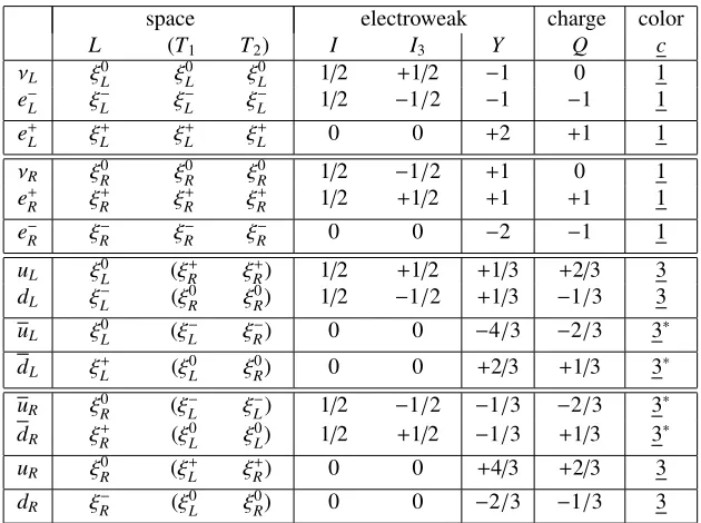
Table 1.Fermionic excitations with their assigments inS O(1,1)×S U(3)CandS O(1,3)×S U(2)I×U(1)Y
symmetry schemes. The column labeled spaceLindicates one of the basic (left/right) modes of the 1D theory (the colored fermionic modes). The columns labeled (T1T2) contain charge eigenstates of two basic modes that
can be combined with theL-mode, giving allowedI3states withinS U(3).
space electroweak charge color
L (T1 T2) I I3 Y Q c
νL ξ0L ξ0L ξ0L 1/2 +1/2 −1 0 1
e−L ξ−L ξL− ξL− 1/2 −1/2 −1 −1 1
e+L ξ+L ξL+ ξL+ 0 0 +2 +1 1
νR ξ0R ξR0 ξR0 1/2 −1/2 +1 0 1
e+R ξR+ ξR+ ξR+ 1/2 +1/2 +1 +1 1
e−R ξR− ξR− ξR− 0 0 −2 −1 1
uL ξ0L (ξ+R ξ+R) 1/2 +1/2 +1/3 +2/3 3 dL ξ−L (ξ0R ξR0) 1/2 −1/2 +1/3 −1/3 3 uL ξ0L (ξ−L ξR−) 0 0 −4/3 −2/3 3∗
dL ξ+L (ξL0 ξ0R) 0 0 +2/3 +1/3 3∗
uR ξ0R (ξ−L ξ−L) 1/2 −1/2 −1/3 −2/3 3∗ dR ξR+ (ξL0 ξL0) 1/2 +1/2 −1/3 +1/3 3∗
uR ξ0R (ξ+L ξ+R) 0 0 +4/3 +2/3 3
dR ξR− (ξL0 ξ0R) 0 0 −2/3 −1/3 3
the instantaneous confining linear potential of the gaugedS U(3) symmetry. In order to study the electroweak structure of quarks (theirvalencenature) one has to study their interactions with the electroweak gauge bosons. This is achieved by mapping the structure of the excitations into three spatial directions in afrozen colorscheme in which we just consider fermions of one particular color (sayr). Take the case of allξRstates with colorrand allξLbeing ¯r. Taking a step back and looking
at what was done in order to find leptons where the frozen colors were in essence space dimensions. The one-dimensional state would be labeled by a single momentum component, which is extended to states labeled by a 3-dimensional momentum vector in E(1,3). For two space dimensions, the fermions could be labeled by their helicity inE(1,2), charge eigenstates being (ξ−ξ−), (ξ+ξ+) and (ξ0ξ0). For leptons in three space dimensions ξ0
L was combined with (ξL0ξ0L) to find an asymptotic
charge eigenstate with (Q,I3) =(0,+1/2), which we already discussed as the left-handed Majorana
neutrinoνL. For colored eigenstates we specify how states are ’viewed’ in 3 dimensions by combining
the (frozen) anti-redξ0
Lstate with the (frozen)rrcombinations (ξR0, ξR0), (ξ+RξR+) or (ξ−Rξ−R). Then only
the combination (ξR+ξ+R) leads to acceptable S U(3) quantum numbers (roots), being an asymptotic acceptableS UI(2) weak eigenstate withI3 =1/2, which hasUQ(1) chargeQ = +2/3, identified as
the weak iso-doublet quark stateuLwith colorrbelonging to a color triplet. Combining the (frozen)
color ¯r stateξ0L with the (frozen)rr¯ combination (ξ0LξR0), (ξL+ξ+R) or (ξ−LξR−) gives only for (ξ−LξR−) an acceptable (frozen) color ¯rstate with (Q,I3)=(−2/3,0), the weak iso-singlet antiquark state ¯uL. The
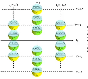
Figure 2.Fermionic excitations and their electroweak quantum numbers for leptons and for quarks (of a given color). Combinations such asξ0
R(ξ 0 Rξ
0 L)
with (I3,Y)=(−1/6,1/3) or ξ0
R(ξ+Rξ+L) with (I3,Y)=(1/6,1)
don’t fit in this scheme.
having two fractionally charged fields (VandT) in 3D, our basic modes are charged or neutral fields living in 1D. The family mixing would also for quarks originate from symmetries in fixing a direction, but in zeroth order there is only a single heavy quark, the top quark (withMt = M), so the mixing
would be simpler. The complete mechanism for masses and mixing for quarks and leptons, however, requires further study.
6 Conclusions
Instead of extending the standard model of particle physics, I have described an attempt to start at a more basic level with just a single space dimension (1D) and as starting point a fully supersymmetric set of three real fields describing bosonic and fermionic excitations. With this supersymmetric, su-perrenormalizable starting point, there is no naturalness or hierarchy problem. TheS O(3) symmetry of the classical ground state, including parity and time reversal, is then in Weyl mode realized as excitations living in 3D. The bosonic degrees of freedom are rearranged into the Higgs particle and the electroweak gauge bosons, while fermions are arranged in three families with two charged (Dirac) and one neutral (Majorana) lepton arranged in left-handed weak isospin doublets and singlets and corresponding right-handed antileptons. All these excitations appear as asymptotic states in 3D. The excitations of the fields also can live in 1D. TheS U(3) gauge theory has an instantaneous confining interaction and no physical gauge degrees of freedom. But this is not how these degrees of freedom show up asymptotically. We argue that the quarks reveal themselves in 3D as good (front form) com-ponents of fractionally charged Dirac fields arranged in a lefthanded weak isospin doublet and two righthanded singlets (and corresponding right- and left-handed antiparticles).
scales for wave-lengths of the one-dimensional excitations producing the right orders of magnitude for masses of top quark, Higgs particle and gauge bosons. There are many details that need to be investigated to see if the proposed scheme can be made consistent, the embedding mechanism for the family structure, the origin of mixing matrices and the emergence of the scale of QCD, where the 1D and 3D descriptions meet. The conjectures as put forward here will likely not invalidate the existing highly successful field theoretical framework for the standard model. Hopefully it could lead to the calculation of parameters as deviations from a zeroth order description. For the QCD part, it also may provide insights why and to what extent collinear effective theories or the many effective theories for QCD at low energies, work. It might provide handles on universality breaking effects such as the ’proton radius puzzle’, the reason being that atomic Hydrogen involves all degrees of freedom of just onefamily while muonic Hydrogen is different in this respect. It could also be interesting to look at more (or maybe less) than three fields, which may also be relevant in the context of the evolution of our universe, in which the world above hadronic scales, i.e. the visible part at nuclear, atomic, molecular scales up to astronomical scales, lives in three space dimensions.
Acknowledgements
I acknowledge useful discussions with several colleagues at Nikhef, in particular Tomas Kasemets. This research is part of the FP7 EU "Ideas" programme QWORK (Contract 320389).
References
[1] J.C. Collins,Foundations of perturbative QCD(Cambridge University Press, 2011) [2] T. Becher, A. Broggio, A. Ferroglia (2014),arXiv:1410.1892
[3] P.J. Mulders,Spin Physics and Transverse Structure, in23rd International Workshop on Deep-Inelastic Scattering and Related Subjects (DIS 2015) Dallas, Texas, United States, April 27-May 1, 2015(2015),arXiv:1508.04244
[4] P.J. Mulders, Operator Structure of TMDs, in Proceedings, QCD Evolution Workshop (QCD 2015)(2015),arXiv:1510.05871
[5] P.J. Mulders,The Roots of the Standard Model of Particle Physics,arXiv:1601.00300 [6] P.A. Dirac, Rev.Mod.Phys.21, 392 (1949)
[7] J.B. Kogut, D.E. Soper, Phys. Rev.D1, 2901 (1970) [8] S.P. Martin, Adv.Ser.Direct.High Energy Phys.21, 1 (2010), [9] J. Wess, B. Zumino, Phys.Lett.B49, 52 (1974)
[10] S.R. Coleman, J. Mandula, Phys.Rev.159, 1251 (1967) [11] N. Cabibbo, Phys. Lett.B72, 333 (1978)
[12] L. Wolfenstein, Phys. Rev.D18, 958 (1978)
[13] E. Ma, G. Rajasekaran, Phys. Rev.D64, 113012 (2001), [14] G. Altarelli, F. Feruglio, Nucl. Phys.B741, 215 (2006), [15] D.B. Kaplan (2013),ArXiv:1306.5818
[16] S. Weinberg, Phys.Rev.D5, 1962 (1972) [17] M. Veltman, Nucl.Phys.B123, 89 (1977)
[18] P. Sikivie, L. Susskind, M.B. Voloshin, V.I. Zakharov, Nucl.Phys.B173, 189 (1980) [19] P.F. Harrison, D.H. Perkins, W.G. Scott, Phys. Lett.B530, 167 (2002),