A MODIFIED FUZZY C MEANS BASED ALGORITHM FOR SEGMENTATION OF MRI IMAGES

DOI: http://dx.doi.org/10.26483/ijarcs.v8i7.4542

Volume 8, No. 7, July – August 2017

International Journal of Advanced Research in Computer Science

RESEARCH PAPER

Available Online at www.ijarcs.info

ISSN No. 0976-5697

A MODIFIED FUZZY C-MEANS BASED ALGORITHM FOR

SEGMENTATION OF MRI IMAGES

Joseph Peter.V

Tamilnadu, India

Abstract: Segmentation is an important process to extract suspicious region from complex medical images. In this research work a new method is proposed to diagnose liver fibrosis and brain tumor through MRI Images using image processing clustering algorithm such as Fuzzy Cognitive Means, along with intelligent optimization tools, such as Hierarchical Self Organizing Map (HSOM), Bacteria Foraging Optimization (BFO). The experimental results of the proposed method are analyzed and compared with other existing methods.

Keywords: Unsupervised classification; Segmentation; MRI Image; Preprocessing; Clustering; Optimization

I. INTRODUCTION

Many algorithms have been proposed for MRI Image segmentation and classification. The most popular methods are included thresholding, region-growing, supervised classification and clustering (unsupervised classification). The full automated intensity-based algorithms have high sensitivity to various noise artifacts such as intra-tissue noise and inter-tissue intensity contrast reduction. Thresholding is very simple and efficient Method. The pre-processing technique eliminates the incomplete, noisy and inconsistent data from the image in the training and test phase. If the images are too noisy or blurred, they should be filtered and sharpened and for removing the unwanted portions of the image. Preprocessing is used to remove the noise. Medical images contain many Gaussian noise and salt and pepper noise. Preprocessing applied in images by using gradient operator method. In preprocessing methods it apply a small neighboring pixel in an input image. Then a new brightness value gets in the output image. This type of preprocessing operations is also called filtration. For preprocessing it use Gradient Operator preprocessing. Basically the Gradient Operators based on local derivatives of the image. At locations of the images the derivatives are bigger. Then the image function undergoes sudden changes. The Objective of the Gradient Operators is to identify such locations in the image. Gradient operators suppress low frequencies in the frequency domain (i.e. they act as high-pass filters). Basically the noise is high frequency in nature. After Applying gradient operator to an image, the noise level in that image increases. Another local pre-processing method is based on the transformation properties [1].

A. Basic Image Processing Operations

Image preprocessing consists of Image histogram equalization, Thresholding, Morphological operation and Region isolation [2]. The first step is to perform histogram equalization on the liver fibrosis and brain MRI image. The given image is equalized using histogram. The Histogram of an image shows the relative frequency of occurrences of pixel in a given image. The non-uniform changeable image due to external conditions is equalized to a uniform variation. Image thresholding image converts an image in 0 to 255 gray levels to a black and white image. The easiest way to use thresholding image is to select a threshold value, and classify all pixels with values above this threshold as white, and all other pixels as black. For this thresholding technique is used. For the equalized image the pixels are represented in a 0 to 255 gray level intensity. As the method is to extract the affected region or the accumulated region, a two level image representation would be satisfactory for better computation. Thresholding often gives an easy and convenient method to achieve this thresholding image on the basis of the dissimilar intensities or colors in the foreground and background regions of an image. For the thresholding image of equalized image a thresholding technique is used as shown below: thresholding image bi, j = 255 if e (i, j) > T Else bi, j = 0 Where e (i, j) is the equalized image and T is threshold resultant for the equalized image.

structuring element of 3x3 matrixes is applied to complete dilation operation. After the dilation operator, a filling operator is used to fill the close contours. Then centroids are calculated to localize the regions as shown beside. The last extracted region is then logically operated for extraction of Massive region in given image.

B. Clustering

Clustering is a simple machine learning technique used to place data elements into related groups without the advanced knowledge of the group definitions. The popular clustering techniques include k-means; Fuzzy C Means (FCM) clustering[3] and Expectation Maximization (EM)[4] clustering. The typical cluster models are Connectivity models, Centroid models, Distribution models. Connectivity model means the hierarchical clustering builds models based on distance connectivity. Centroid model means the K-means algorithm represents each cluster by a single mean vector. Distribution model means the clusters are modeled using statistic distributions, such as multivariate normal distributions used by the Expectation-Maximization algorithm. A clustering is generally and essentially a set of such clusters usually containing all the various objects in the data set. Additionally, it may clearly specify the relationship between the clusters to each other, for example, a hierarchy of clusters embedded in each other. The clustering can be mainly distinguished in hard clustering and soft clustering or fuzzy clustering, where each object belongs to each cluster to a certain degree.

C. UNSUPERVISED LEARNING

Unsupervised learning is nothing but input patterns where no external teacher is present and Self organisation is showing patterns to be classified, network produces own output representation. Three properties required. The value of output used as measure of similarity between input pattern and pattern stored in neuron. Competitive learning strategy selects neuron with largest response and Methods of reinforcing largest response. In Self Organizing Map (SOM)[5], units located physically next to one another will respond to input vectors that are similar. SOM uses unsupervised learning to physically arrange its neurons so that the patterns that it stores are arranged such that similar patterns are close to each other and dissimilar patterns are far apart.

Hierarchical Self Organizing Map (HSOM)[6] is an algorithm that finds a solution to an optimization problem. It is the combination of self organization and graphic mapping technique.

The HSOM is organized in a pyramidal mannered structure consisting of multiple layers where each layer resembles the single layer of SOM. HSOMs are very easy to understand and they are simple. HSOM is used to classify data accurately and easily evaluate for their own quality. Learning process has sequential corrections of the vectors representing neurons. On every step of the learning process a random vector is chosen from the initial data set and then the best matching neuron

coefficient vector is identified. The most similar to the input vector is selected as a winner or optimal threshold value.

II. LITERATURESURVEY

The digital image processing community has developed several segmentation methods, four of the most common methods are: 1) amplitude thresholding, 2) texture segmentation 3) template matching and 4) region-growing segmentation. It is very important for detecting tumors, edema and necrotic tissues. These types of algorithms are used dividing the brain images into three categories (a) Pixel Based, (b) Region or Texture Based and (c) Structural Based.

Several authors suggested various algorithms for segmentation. Chunyan et al. described a deformable method for segmenting MRI images semi automatically [7]. Tsai et al. presented a method on Histogram and Morphological operation for segmenting the various tissues from MRI data [8]. Daniel et al. designed Statistical Validation of Brain Tumor Shape Approximation via Spherical Harmonics for Image Guided Neurosurgery [9]. Jayaram et al. represented Fuzzy Connectedness and Fuzzy sets used to develop the concept of fuzzy connectedness directly on the given image for facilitating the image segmentation [10-11]. Hideki et al. specified a technique to Partition the image space into meaningful regions [12]. Benedicte et al designed a method on Expectation-maximization (EM) for segmenting white matter (WM), gray matter (GM) and colony stimulating factor (CSF) [13]. Jing et al. described fuzzy model to design the fitness function of Gas and to guide the region growing [14]. Kabir et al. prescribed Markov random field model for segmenting stroke lesions on MR Multi sequences [15]. Tang et al. presented Multi resolution image segmentation for segmenting the brain tissue structure from MRI [16]. Pierre et al. prescribed Atlas-based segmentation for Propagation of the labeled structures to the MRI [17] Siyal et al described a new method on Fuzzy C-means for segmentation purpose. Aaron designed level set surface model for GUI based segmentation [18]. Mark et al. designed a Segmentation of Brain Tumors using Alignment-Based Features [19]. Markey et al. (2003) identified and characterized clusters in a heterogeneous breast cancer computer-aided diagnosis database [20-21]. Identification of subgroups within the database could help elucidate clinical trends and facilitate future model building. A self-Organizing map (SOM) was used to identify clusters in a large, heterogeneous computer-aided diagnosis database based on mammographic findings (BI-RADSTM) and patient age.

III. PROPOSEDMEHOD

Tumor pixels were detected using the Hierarchical Self Organizing Map with FCM approach. It is concluded that the proposed approach has finding higher Tumor value and lesser execution time than SOM.

The HSOM and FCM are very simple, easy to understand and they work well. Here the main drawback of HSOM is to detect the number of cluster to be specified and the data set is not known in the priori. So to overcome the problem the population based Bacteria Foraging Optimization Algorithm (BFOA) algorithm [22] is used to solve the chromosome encoding with multiple solutions. Tumor is an abnormal growth in the liver fibrosis caused by cells reproducing themselves in an uncontrolled manner. The radiographer is usually responsible for acquiring medical images of diagnostic quality, although some radiological interventions are performed by radiologists. Our system reduces the involvement of radiologists in detecting the Tumor and helps the radiographer to provide a secondary opinion with a considerable rate of accuracy. Obtaining real medical images for carrying out research is highly difficult due to privacy issues, legal issues and technical hurdles. Hence, the UCI Machine learning database is used in this thesis to study the efficiency of the proposed intelligent system since it is a benchmark database available online for research. And also medical images are taken from KMCH Hospital, Coimbatore, Tamilnadu, India.

A. FUZZY C MEANS CLUSTERING ALGORITHM

The traditional Fuzzy C Means (FCM) clustering algorithm works simply by assigning membership to each data point corresponding to each cluster center on the basis of the distance between the cluster center and the data point. When the data is near to a cluster center, its membership towards the cluster centre is considered to be correlated. Here, the summation of the membership of each data point should be equal to one. After each iteration, the membership and cluster centers are

updated according to the equation (1)

(1) where n is the number of data points, vj is the jth cluster center, m is the fuzziness index m ɛ [1, ∞], c is the number of cluster center, μij is the membership of ith data to jth cluster center and dij is the Euclidean distance between ith data and jth cluster center. The main objective of the fuzzy c-means algorithm is to minimize:

(2)

Where ||xi – vj|| is the Euclidean distance between ith data and jth cluster center. The algorithmic steps for the Fuzzy c-means clustering are given below,

Let X = {x1, x2, x3 ..., xn} be the set of data points and V = {v1, v2, v3 ..., vc} be the set of centers.

1) Randomly select ‘c’ cluster centers.

2) Calculate the fuzzy membership 'μij' using equation (1) 3) Compute the fuzzy centers 'vj' using equation (1)

4) Repeat Steps 2 & 3 until minimum j value is achieved or ||U(k+1) - U(k)|| < β.

Here, k is the iteration step, β is the termination criterion between [0, 1],

U = (μij)n*c is the fuzzy membership matrix and j is the objective function.

The algorithm has several advantages as listed below.

1. FCM gives the best result for the overlapped dataset and comparatively better than the k-means algorithm.

2. Unlike the k-means where the data point must exclusively belong to one cluster center, here the data point is assigned membership to each cluster center as a result of which the data point may belong to more than one cluster center.

These advantages make the fuzzy c means a more frequently used clustering algorithm. However, the following points can be improved to enhance the algorithm much more. Specification of the number of clusters (k), Choice of distance measure (d) Choice of fuzziness parameter (m), Estimation of the termination criteria (β)

Choice of fuzziness parameter:

Generally, the value of the fuzzifier, m, is set equal to two. This can be considered a compromise between an assumption of a certain amount of fuzziness in the dataset and the advantage of avoiding a time consuming calculation of its value. However, by adjusting the fuzzifier carefully, it must be possible to optimize the algorithm. The proposed optimization procedure is termed as the Automatic Fuzziness Parameter Estimator (AFPE).

B. Estimation of the termination criteria (β) :

The termination condition in the FCM uses a threshold value (β) and the clustering process stops only when the differences between the centers of the clusters of two successive iterations is less than or equal to this threshold value. This traditional method has the following disadvantages as seen below:

• There is a strong chance that the iterations might never reach the threshold value which leads to an infinite loop.

• The iterative process might also produce a value very close to the threshold. The algorithm does not recognize this as stabilized state and continues till the values are exactly equal. This scenario results in the waste of time and resources and increases the complexity of the algorithm.

• According to the traditional algorithm, when m→∞, then the degree of the membership function of xi in cluster j is 1/K. Thus the upper bound of m is set as 1/K.

• In order to achieve strongly related clusters, the membership values should be high, even for low m values (m<2).

• In order to achieve this estimator the procedure given below is used.

o Mub = 1/K o M = 1 + m0

o m0 = 1 mub ≥ 10 o M0 = mub/10 mub < 10

• This procedure makes sure that the m value is above 2 for mub greater than 10 and m < 2 when mub < 10 and never goes to ∞.

This traditional method has the following disadvantages as seen below:

• There is a strong chance that the iterations might never reach the threshold value which leads to an infinite loop.

• The iterative process might also produce a value very close to the threshold. The algorithm does not recognize this as stabilized state and continues till the values are exactly equal. This scenario results in the waste of time and resources and increases the complexity of the algorithm.

To solve the above mentioned issue, this study uses a modified membership function that uses the fuzzy logic concept and is termed as the Automatic Termination Criteria Estimator (ATCE) and the procedure is given below:

• Create a fuzzy set S as a set of clusters {cj, μj}, where cj is the cluster center which is almost equal to the previous cluster center cj−1 and μj is the degree of the membership. The degree of closeness is calculated as follows :

(3) where d1 is the distance between 2 cluster centers and dmax1 is the maximum distance obtained during the first iteration. The values d1 and dmax1 will be the same initially and dmax1 is continuously evaluated and adjusted during each iteration and hence are dynamic in nature. The algorithm terminates when the following three conditions are met When the degree of closeness between the cluster and the fuzzy set S is > 0.9 Till the degree of closeness of current < previous iteration’s degree of closeness, even if the current degree of closeness is > 0.9. Due to its design the extended approach of the FCM is as powerful as the existing and it is safer in the sense that it is never involved in an infinite iterative process.

C. SELF-ORGANIZING MAP

The SOM is used to detect the Tumor region with minimum intensity and similar Tumor region which is given by SOM

from the given image using FCM method. A self-organizing map (SOM) or Self-Organizing Feature Map (SOFM), commonly also known as Kohonen network, is a type of Artificial Neural Network (ANN) that is trained using unsupervised learning to produce a low-dimensional, discretized representation of the input space of the training samples, called a map. Self-Organizing Maps are different than other artificial neural networks in the sense that they use a neighborhood function to preserve the topological properties of the input space. Like most Artificial Neural Network, SOMs operate in two modes: training and mapping. Training builds the map using input examples. It is a competitive process, also called vector quantization. Mapping automatically classifies a new input vector.

A self-organizing map consists of components called nodes or neuron. Associated with each node is a weight vector of the same dimension as the input data vectors and a position in the map space. The arrangement of nodes is a regular spacing in a hexagonal or rectangular grid. The self-organizing map describes a mapping from a higher dimensional input space to a lower dimensional map space. The procedure for placing a vector from data space onto the map is to find the node with the closest weight vector to the vector taken from data space and to assign the map coordinates of this node to our vector.

The goal of learning in the self-organizing map is to cause different parts of the network to respond similarly to certain input image patterns. The weights of the neurons are initialized either to small random values or sampled from the subspace spanned by the two largest principal component eigenvectors. With the latter alternative, learning is much faster because the initial weights already give good approximation of SOM weights. The network must be fed a large number of vectors that represent, as close as possible, the kinds of vectors expected during mapping. In this thesis the training utilizes competitive learning. When a training image patterns are fed to the network, its Euclidean distance to all weight vectors is computed. The neuron with weight vector most similar to the input is called the Best Matching Unit (BMU).

1 Randomize the map's nodes' weight vectors; 2 Grab an input vector;

3 Traverse each node in the map

4 Use Euclidean distance to find similarity between the input vector and the map's node's weight vector;

5 Track the node that produces the smallest distance (this node is the Best Matching Unit, BMU);

6 Update the nodes in the neighborhood of BMU by pulling them closer to the input vector; Increment n and repeat from 2 while n < N.

neuron: the neuron whose weight vector lies closest to the input vector.

IMPLEMENTATION OF SOM with FCM:

The winning neuron equation of SOM giving input to the FCM Based on the previous equation, the first step of the regularized FCM-SOM algorithm is the following:

Step 2: Calculate the cluster centers. C = (N/2)1/2 Step 3: Compute the Euclidean distances Dij = CCp – Cn Step 4: Update the partition matrix (Repeat the step 4) Until Max [│Uij (k+1)-Uijk│] <€ is satisfied

Step 5: Calculate the average clustering points. Step 6: Compute the adaptive threshold

Adaptive threshold =max (Adaptive threshold, ci) i=1...n In the first step, the algorithm selects the initial cluster from HSOM Clustering algorithm. Then, in later step after several iteration of the algorithm, the final result converges to actual cluster center achieved and it is very important for an FCM algorithm.

D. HSOM WITH FCM

HSOM is the combination of Self organization and tomography mapping techniques. The HSOM is organized as a pyramid structure consisting of multiple layers where each layer resembles the single layer of SOM. In the Algorithm of HSOM with FCM, Liver fibrosis Image is given as Input and Segmented Image contain only Tumor (suspicious region) should be an Output. The optimal value of HSOM through Liver fibrosis Image is given as an input for FCM The Winning neuron formula Wn = ||x-Wc||=Max {[x-Wi]} Where x is the neuron, Wc is the Winning neuron, Wi is the Weight vector. In this winning neuron equation the output ie optimal value of HSOM giving input to the FCM. The Maximum Adaptive threshold value is used to compare the current neuron value. If the current value is less than the Adaptive Thresholds neglects the region set to black and the suspicious region is look like bright.

E. BFOA WITH FCM

Foraging strategies denote the phenomenon of search, handling and ingestion of nutrients. The implementation of the Bacterial Foraging Optimization algorithm, which is a modern global optimization tool using iterative stochastic searches, is a computational analogue of the behaviour of intestinal bacteria in their search for nutrients in a hostile environment with minimal loss in energy.

Markov Random Field (MRF)

The MRI image is stored in a two-dimensional matrix and a kernel is extracted for each pixel. A unique label is assigned to the kernels having similar patterns. In the labeling process, a label matrix is initialized with zeros. The size of the label matrix is equal to the size of the MRI image. For each pixel in the image, the label value is stored in the label matrix at the location corresponding to its central pixel coordinates in the gray level image. A pattern matrix is maintained to store the dissimilar patterns in the image. For each pixel, a kernel is extracted and the kernel is compared with the patterns

available in the pattern matrix. Once it finds any matches the same label value is assigned to the currently extracted kernel. Otherwise the next label value is assigned to the kernel and the kernel is added to the pattern matrix. The labels are assigned integer values starting with one and incremented by one whenever a new pattern occurs.

Finally the pattern matrix contains all the dissimilar patterns in the image and the corresponding label values are also extracted from the label matrix. For each pattern in the pattern matrix, the posterior energy function value is calculated using the equation (4).

(4) The challenge of finding the MAP estimate of the segmentation is to search for the optimum label which minimizes the posterior energy function U(x).

multi-dimensional search space, making best use of previous best positions encountered by itself, as well as other members of the population.

The BFO technique iteratively optimizes a given objective by sharing mutual information about the optimality of each of the previously encountered points on the search space in order to finally arrive at a global optimum. The BFO algorithm comprises four stages, namely: Chemotaxis, Swarming, Reproduction and Elimination-Dispersal. BFO performs these four actions iteratively to obtain a global optimum. The bacterial foraging procedure is briefly presented. A full and detailed mathematical discussion can be found. Let ᶿ ∈ Rp , where Rp denotes a p-dimensional vector of real numbers which is a trial solution in the search space and J(ᶿ) be any objective function whose global optimum is of interest and whose gradient may not be determined analytically. Different values of the function denote different conditions of the nutrient surface in the search space which the bacteria currently occupy. Negative, zero and positive values of J (ᶿ) represent nutrient-rich, neutral and noxious gradients, respectively. Hence, the aim of the BFO is to minimize the objective function to facilitate bacterial growth.

The optimal value of BFO giving input to the FCM. The algorithm selects the initial cluster from BFO Algorithm. Then, in later step after several iteration of the algorithm, the final result converges to actual cluster of BFO with FCM. The aim of BFO with FCM is to detect the suspicious region from the background region in the MRI brain and liver fibrosis Image. The Maximum Adaptive threshold value is used to compare the pixel value. If the pixel value is less than th23e Adaptive Thresholds neglects the region set to black and the suspicious region is look like bright.

Implementation of BFO with FCM

The optimal value of BFO giving input to the FCM. The aim of FCM is to find cluster centers (centroids) that minimize dissimilarity function. The membership matrix (U) is randomly initialized as

(5)

where i is the number of cluster, j is the image data point The dissimilarity function can be calculated with this equation

c(6) where Uij is between 0 and 1,Ci is the centroid of cluster i, dij is the Euclidean distance between ith and centriod (Ci ) and jth data point, M is a weighting exponent.

To calculate Euclidean distance (dij)

Euclidean distance (dij) =

Cluster center pixels - current neuron

Dij = CCp – Cn where CCp is the Cluster center pixels, Cn is the current neuron i.e. Number of clusters is computed as C = (N/2)1/2

N= no. of pixels in image

The Minimum dissimilarity function Uij can be computed as

(8) where dij=||xi -cj|| and dkj=|| xi –ck||, xi is the ith of d- dimensional data, cj is the d-dimensional center of the cluster, ||**|| is the similarity between any measured data and center, so, these iteration will stop when the condition is satisfied

(9) where € is a termination criterion between 0 and 1, K is the iteration step.

The step of the FCM Algorithm has been listed Step 1: Initialise U = Uij matrix

Step 2: At K step initialize centre vector C (k) = C j taken from GA Clustering algorithm

Step 3: Update U (k), U (k+1), then compute the dissimilarity function using (8). If || U (k+1) - U (k) || < € then stop. Otherwise return to step3.

Input: MRI Image

Output: Segmented image contain only Tumor (suspicious reign)

Step 1: The optimal value of BFO giving input to the FCM. FCM- BFO Algorithm is the following:

Step 2: Calculate the cluster centers. C = (N/2)1/2 Step 3: Compute the Euclidean distances Dij = CCp – Cn Step 4: Update the partition matrix using (8)

(Repeat the step 4)

Until Max[ │Uij(k+1)-Uijk│] <€ is satisfied Step 5: Calculate the average clustering points using (6). Step 6: Compute the adaptive threshold

Adaptive threshold =max (Adaptive threshold, ci ) i=1...n The Maximum Adaptive threshold is used to compare the current neuron value. If the current value is less than the Adaptive Thresholds then the region set to black and the suspicious region is look like bright.

IV. EXPERIMENTSANDRESULTS

Fig. 1 shows the Input images such as MRI Liver and MRI Brain. In the existing system, for segmentation of tumor it use BFO and 2D Otsu[23] method .Otsu is used to generate the function to be optimized, ABC[24] is applied to determine the optimized values of threshold parameters. This existing system is time consuming. It takes large amount of computation time. So in this work a new method is introduced for the segmentation and classification of tumor from an MRI images. This method contains the combination of BFO and FCM. This method results lower computation time and better performance than existing method.

Fig 1. Input MRI Liver Fibrosis Image and MRI Brain Image

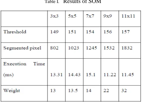
A. Results of SOM

Liver fibrosis and MRI brain Image is given as Input and segmented by using SOM. All pixel of an Image are represented in a 256x256 matrix. In this experiment consider a part of the Image. let us consider 5x5 matrix to find the Winning neuron (optimal value). The SOM Weight vector is needed to find out the overall given Image value for 3x3, 5x5, 7x7, 9x9 and 11x11.The Winning neuron is calculated using Weight vector matrix. The table I shows that the Adaptive threshold for 3x3 is 149, 5x5 is 151, 7x7 is 154, 9x9 is 156 and 11x11 is 157. Also it shows the Number of Segmented Pixels, Execution time and Weight.

Table I. Results of SOM

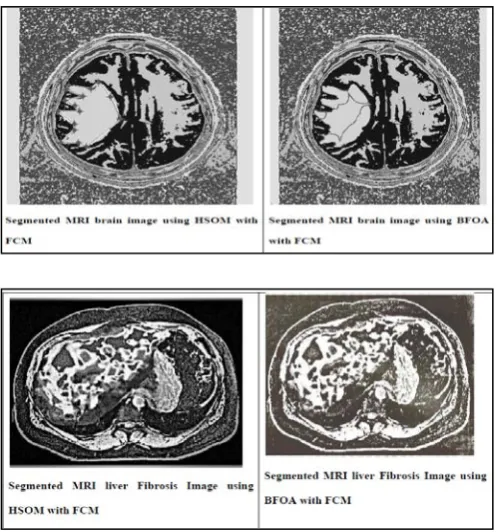
B. Results of HSOM with FCM

The aim of HSOM with FCM is to detect the suspicious region from the background region in the MRI brain and liver fibrosis Image. In this experiment consider a part of the image which is

the 9x9 matrix in Table III. The main aim of FCM is to minimize Dissimilarity function. The Winning neuron through MRI Image is giving as an input for FCM. Adaptive threshold: Wn = ||x-Wc||=Max {[x-Wi]}. After solving the equation the Winning neuron is obtained.

Table II. Results of HSOM with FCM

Value/Neighbourhood pixel

3X3 5X5 7X7 9X9 11X11

Adaptive Threshold 175 171 170 149 146

Number of Segmented 795 1294 1947 3413 7400

Execution Time (MS) 11 23 24 27 30

Weight 23 23.5 24 32 42

Similarly to find the overall given Image value for 3x3, 5x5, 7x7, 9x9 and 11x11 the Winning neuron is calculated using Weight vector matrix. The table II shows that the Adaptive threshold, segmented pixels, execution time and weight.

Table III. 9x9 Digitized Intensity Matrixes

performance of the MRI Image in terms of Weight vector, Execution Time and Tumor Pixels detected using the Hierarchical Self Organizing Map with FCM approach, it can be concluded that the proposed approach has lower Tumor value and lesser execution time.

The FCM classification algorithm for MR images segmentation, which may performs very fast and simple, but this algorithm do not guarantee high accuracy especially for noisy or abnormal images. Unfortunately, MR images always contain a significant amount of noise caused by operator, equipment, and the environment, which lead to serious inaccuracies in the segmentation. So this introduced FCM before performing BFO classification algorithm, in order to avoid sensitivity to noise. Fig. 2 shows the segmented image. The segmented image doesn’t give accurate solution. After classification it classify tumor in an image. After segmentation identifies the tumor infected region. So before classification select the tumor region and then perform classification.

Fig. 2. Segemented MRI Images using FCM

In Fig. 3, the selected region shows the tumor infected region. Then it performs many iterations. The final result shows the exact tumor region.

Fig. 3. Segemented MRI Images after Classification

Results of BFO with FCM

In all pixel of an image are represented in a 256x256 matrix. In this experiment we consider a part of the image which is the 9x9 matrix as in table IV. Let us consider an example,

Table IV. 9x9 Digitized Intensity Matrixes

The Global optimal value of BFO is sent through Image is given as an input for FCM to find the overall given image value for 3x3, 5x5, 7x7, 9x9 and 11x11.The Winning neuron is calculated using Weight vector matrix, Number of Segmented Pixels, Execution time and Weight.

The Maximum Adaptive threshold is used to compare the current neuron value. If the current value is less than the adaptive Thresholds neglects the region set to black and the suspicious region is look like bright. So the entire image in sliding window to detect the suspicious region from the background region.

C. Performance Analysis

It is very difficult to measure the performance of enhancement objectively. If the enhanced image can make observer perceive the region of interest better, then we can say that the original image has been improved. Here are giving input image in that neighborhood pixel of 3×3, 5×5, 7×7, 9×9 and 11×11 windows are analyzed. In that 3×3 window is chosen based on the high contrast than 5×5, 7×7, 9×9 and 11×11. Results in Table V show the Execution time, number of segmented pixel, Adaptive Threshold and for HSOM with FCM and BFO with FCM.

A Fuzzy C Means with BFO based Segmentation process to detect MRI brain and Liver fibrosis Tumor was implemented. In that performance of the Image in terms of Weight vector, execution time and Tumor pixels detected using the BFO with FCM approach, it can be concluded that the proposed approach has lower Tumor value and lesser execution time. There is a decrease in both the values when compared to any other existing approach [25-26].

In the existing system, for segmentation of tumor it use BFO and 2D Otsu method .Otsu is used to generate the function to be optimized, ABC is applied to determine the optimized values of threshold parameters. This existing system is time consuming. it take large amount of computation time. So in this introduce a new method is used for the segmentation and classification of tumor from an MRI images. This method contains the combination of BFO and FCM. This method results lower computation time and better performance than existing method. In future plan to investigate the different aspects of medical imaging which can be formulated as optimization problems and develop effective methods.

One of the oldest methods for image segmentation is due to Otsu. This method though popular and reasonably effective has a drawback that it is computationally very costly. A novel method for the supervised and unsupervised classification and grading of liver fibrosis based on hepatic hemodynamic changes measured noninvasively from functional MRI scans combined with ypercapnia and hyperoxia. The supervised learning methods such as BFO and FCM automatically create a classification and grading model for liver fibrosis grade from training datasets.

V. CONCLUSION

This research work highlights the Pre-Processing, Enhancement, Clustering, FCM, HSOM with FCM and BFOA with FCM methods. The algorithms are used to identify the tumor in the affected area. The experimental results of various methods are analyzed. The results show that the proposed method BFOA with FCM can perform better than other existing methods.

VI. REFERENCES

[1] Nock, R. and Nielsen, F. (2006) "On Weighting Clustering", IEEE Trans. on Pattern Analysis and Machine Intelligence, 28 (8), 1–13.

[2] Gonzalez, R.C. and R.E. Woods, “Digital image processing, Pearson Education”, 2002.

[3] Siyal M.Y, Lin yu (2005),”An Intelligent modified fuzzy C-means based algorithm for bias estimation and segmentation of brain MRI”,Elsevier,Pattern Recognition Letters,26.

[4] Wu, C. F. Jeff (Mar. 1983). "On the Convergence Properties of the EM Algorithm". Annals of Statistics 11 (1): 95–103.

[5] Mia K. Markeya,b,*, Joseph Y. Loa,b ,Georgia D. Tourassib , Carey E. Floyd Jr.a,b, Selforganizing map for cluster analysis of a breast cancer database",Artificial Intelligence in Medicine 27 (2003) 113–127

[6] Michael Dittenbach, Dieter Merkl, Andreas Rauber, Growing hierarchical self-organizing map, Proceedings of the Int’l Joint Conference on Neural Networks (IJCNN’2000), Como, Italy, July 24-27, 2000, pp VI-15 - VI-19.

[7] Chunyan Jiang, Xinhua Zhang, Wanjun Huang,Christoph Meinel.:”Segmentation and Quantification of Brain Tumor,”IEEE International conference on Virtual Environment,Human-Computer interfaces and Measurement Systems, USA, 12-14, July 2004.

[8] Tsai Y-C., C-H.Cheng and J-R.Chang, Entropy-Based Fuzzy Rough Classification Approach for Extracting Classification Rules, Expert Systems with Applications, 1-8, 2005.

[9] Daniel Goldberg-Zimring, Ion-Florin Talos, Jui G.Bhagwat, Steven J Haker, Peter M.Black, and Kelly H.Zuo,:”Statistical Validation of Brain Tumor Shape Approximation via Spherical Harmonics for Image Guided Neurosurgery”.

[10] Jayaram K.Udupa,Punam K.Saha,:”Fuzzy Connectedness

and Image Segmentation”, Proceedings of the IEEE,vol.91,No 10,Oct 2003.

[11] Jayaram K.Udupa, Vicki R.Lablane, Hilary

Schmidt,Celina Lmielinska, Punam K.Saha,George J.Grevera,Ying Zhuge,Pat Molholt,Yinpengjin,Leanne M.Currie,:”A Methodology for Evaluating Image Algorithm”,IEEE on Medical Image Processing.

[12] Hideki yamamoto and Katsuhiko Sugita, Noriki Kanzaki,

Ikuo Johja and Yoshio Hiraki,Michiyoshi Kuwahara , : “Magnetic Resonance Image Enhancement Using VFilter”, IEEE AES Magazine, June 1990.

[13] Benedicte Mortamet,Donglin Zeng,Guido Gerig,

[14] Jing-hao Xue,Su Ruan,Bruno Moretti,Marinette Revenu,Daniel Bloyet,:”Knowledge-based Segmentation And Labeling of brain structure fromMRI images”,Elsevier,Pattern Recognition Letters 22,2001.

[15] Kabir.Y, Dojat.M, Scherrer.B, Forbes.F,

Garbay.C:”Multimodal MRI Segmentation of ischemic stroke Lesions”,April 2007.

[16] Tang H, Wu E.X, Ma Q.Y, Gallagher D Perera G.M,

Zhuang T,:”MRI brain image segmenatation by multi- resolution edge detection and region selection”,Pergamon on Computerized Medical imaging and graphics 24,2000.

[17] Pierre-Yves Bondiau,Gregoire Malandain, Stephane

Chanalet,Pierre-Yves Marcy,:”Atlas-Based Automatic Segmentation of MR Images:Validation Study on The Brainstem in Radiotherapy Context”,Elsevier on radiation Oncology Biological Physis,vol.61,2005.

[18] Siyal M.Y,Lin yu,:”An Intelligent modified fuzzy

C-means based algorithm for bias estimation and Segmentation of brain MRI”,Elsevier,Pattern Recognition Letters,26,2005.

[19] Mark Schmidt, Ilya Levner, Ressell Greiner, Albert

Murtha, Aalo Bistritz,:”Segmentation Brain Tumors using Alignment-Based Features”,IEEE on Proceesings of the fourth International Conference on Machine Learning an Applications(ICMLA’05)”,2005.

[20] Mia K. Markeya,b,*, Joseph Y. Loa,b ,Georgia D.

Tourassib , Carey E. Floyd Jr.a,b, "Selforganizing map for cluster analysis of a breast cancer database",Artificial Intelligence in Medicine 27 (2003) 113–127

[21] Markey MK, Lo JY, Floyd Jr. CE. Differences between

computer-aided diagnosis of breast masses and that of calcifications. Radiology 2002;223:489–93.

[22] S. Das and A. Biswas and S. Dasgupta and A. Abraham,

"Bacterial Foraging Optimization Algorithm: Theoretical Foundations, Analysis, and Applications", in Foundations of Computational Intelligence Volume 3: Global Optimization, pages 23–55, Springer, 2009.

[23] Jun Zhang and Jinglu Hu, Image Segmentation Based on

2D Otsu Method with Histogram Analysis, International Conference on Computer Science and Software Engineering, 2008.

[24] D. Karaboga, B. Basturk Akay, C. Ozturk, Artificial Bee

Colony (ABC) OptimizationAlgorithm for Training Feed-Forward Neural Networks, LNCS: Modeling Decisions for Artificial Intelligence, Vol: 4617/2007, pp:318–319, Springer-Verlag, 2007.

[25] S. Mishra. A Hybrid Least Square-Fuzzy Bacterial

Foraging Strategy for Harmonic Estimation. February 2005.

[26] Muñoz, M A. Simplifying the Bacteria Foraging