International Journal of Advanced Research in Computer Science
TECHNICAL NOTE
Available Online at www.ijarcs.info
Comparison Analysis of Time Series Data Algorithm Complexity for Forecasting of
Dengue Fever Occurrences
Faculty of Math and Natural ScienceYogyakarta, Indonesia
Abstract: Times series complexity is a testing standard of a particular algorithm to achieve efficient time execution when it is implemented into programming language. Complexity of the algorithm is differentiated into two parts; those are time series complexity and space complexity. Time series complexity is determined from the numbers of computation steps needed to run algorithm as a function of several data n (input size). However, space series complexity is measured from the memory used by data structure found in the algorithm as the function of several data n. The objective of the study is to test the comparison of three forecasting algorithms among time series complexities by using operational empirical analysis with running time application when the algorithm is used in programming language or a particular application. The algorithms tested in this study were Linear Regression, SMO Regression, and Multilayer Perceptron by using Weka Application. The analysis result and the test result all three algorithms showed that running time was significantly influenced by algorithm’s complexity and additional data set numbers that became the input. Furthermore, running time analysis from those three algorithms showed stable rate respectively from SMO Regression, Linear Regression, and Multilayer Perceptron. However, for Big-O algorithm analysis Linear Regression and SMO Regression had almost similar time complexity, but they had far different from Multilayer Perceptron that tended to be more complex.
Keywords: time complexity, time series data, linear regression, SMO Regression, multilayer perceptron, Big-O
I. INTRODUCTION
Time series forecasting (TSF) is a technique to predict the future based on the variables that have been observed before [1][2]. Forecasting model has been used extensively in some applications such as health, financial, share market, information technology, and many more. Generally, the phenomena of using tie series data has its limitation toward forecasting because the information achieved is limited to the values in the past from its data series. During the last several decades, there are more various interests and understandings in predicting the future. Most methods used by the users lean on linear model and non-linear statistical model. Linear statistical model is easily explained and implemented; this model is suitable for time series data coming from non-linear process. Linear statistical model has a limitation [3] on its linear part, so this model has a limitation on problem solving TSF in the real field. In further, the equation process of non linear statistical model toward TSF problems is an activity that is difficult to execute [4].
In addition, to understand the level of complexity toward an algorithm, people need to have a test and comparison toward several algorithms. In this study, the researchers are going to explain and investigate the comparison of complexity and computability level of time series forecasting algorithm on the data of dengue fever occurrences. Three algorithms that are used as the subjects of comparison are linear regression, sequence minimum optimization (SMO) and multilayer perceptron.
II. LITERATUREREVIEW
A. Linier Regression
The purpose of regression analysis is to find out forecasting result of data time series in the future based on the value of observation that will be the sample of the data. In another word, if the value is n from the sample achieved as the predictor, yn + 1 will be predicted based on the input, while xn + 1 is the result of sample analysis. When the process of regression model is yielded, the process of data item forecasting is done based on the stream of regression data model which becomes a time organization for every data counted on the number of total occurrences. In conducting reorganization, the data is gathered as similar input and counted the time difference when the data is obtained. In further, cluster the data based on the time series by counting while doing data reorganization. Here it the algorithm [5]: a. Giving the data input as the input data with N size and
threshold.
b. Counting the forecasting, in which forecasting value is not more than the threshold.
c. Determining time series as an independent variable and the number of occurrences dengue fever data as a dependent variable.
b
^0=
y
- b
^1x
……….. (2)
……….. (3)
e. Adjusting the regression model.
y=b
0+ b
1+ ε
……….. (5)
f. Counting the equation’s error
ε1
=y
1-y^
1……….. (6)
B. SMO Regression
SMO Regression algorithm is based on the algorithm of Sequence Minimum Optimization (SMO) to overcome regression problem. Regression analysis is a mathematical statistical method used to handle the correlation among variables, that is able to break down prediction problem [6]. Sequence Minimum Optimization is simple machine learning algorithm that can solve Support Vector Machine (SVM) Quadratic Programming (QP) quickly without saving extra matrix and without involving repeated numerical routine for every problem. SMO chooses to solve the smallest optimization possibility in its every step. For standard problem SVMQP, the possibility of the smallest optimization problem involves two Lagrange Multipliers because Lagrange Multipliers should follow linear equivalent.
Here it is the algorithm of Sequence Minimum Optimization:
a. Giving data set sample to conduct data training, b. At the first time, SMO is used to count the limit of
multipliers, in further determining the minimum limit, with the equation:
L=max(0, α2 – α1), H=min(C, C + α2 – α1).
……….. (7) c. If target y1 is similar to y2, these following limit work
for α2;
L=max(0, α2 + α1 - C), H=min(C, α2 – α1)
……….. (8) d. The second differential from objective function can be
expressed, as follow:
η =K(x1, x1)+ K (x2, x2)- 2 K(x1, x2)
……….. (9) e. In a normal condition, objective function will have
positive value. In this case, it will have minimum value as long as the linear pointer is same as the limit,
and η is bigger than nol. In this case, SMO counted the minimum with this following limit:
……….. (10) f. The next step is to find out the minimum limit by
clipping to minimum line that is not limited until the edge of the top line;
……….. (11)
g. Counting the value s=y1y2 with value α1 counted from
new clipping α2 ;
……….. (12)
C. Multilayer Perceptron
To conduct time series prediction with classical method, there are several steps that should be followed. Those steps consist of time series analysis, time series model, model identification, and parameter estimation. In conducting those following steps, there are some obstacles such as [7]:
a. There are some messed up data series;
b. The data result is taken from observation, so it is possible to make mistake of measuring that will influence the result of prediction.
c. Data series has various behavior
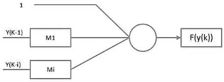
Artificial neuron receives the input signal to make prediction y(k-i) while i=input number, the input will be transmitted through the equation i+1 to get the scale, and then the scale of the input is a linear combination from output signal that has obtained activation function. The model of neuron illustration can be seen in Figure 1.
Figure 1. Ilustration of artificial neuron for prediction (M1 and i is multiplier)
The sample of time series data can be symbolized with x(t) that is gathered to build a prediction of the model. Sample data x(t) in data series gives time k as its step. Time series value prediction can be made by using one step ahead, this step is used to find out the best estimated value.
Multilayer perceptron is a popular machine learning algorithm in the network of artificial neuron that can give an output suitable its training to the network as well as to have coefficient calculation with the closest distance. To conduct data training, people need to have a particular algorithm for a multi-layer network.
a. Use data set sample as the input of data training to make the network pattern.
{ }
output unit on layer N. Layer connection is connected by (n) on the previous layer which is layer (n-1) given value
.
c. Value initiation, the example: put range between [–smwt, + smwt].
d. Forecasting selection error uses the function f= and
n learning rate.
e. Update value with equation Δ to achieve
the value from every training pattern p. One update
set value toward the whole training pattern is mentioned with 1 epoch training.
f. Repeat step 5 until the network get “small” error function.
III. RESEARCHMETHOD
The research is started by gathering related literature review with the algorithm that will be compared and analyzed its complexity by using Big-O for three algorithms, Linear Regression, SMORegression, and Multilayer Perceptron. In further, the algorithm is tested by using Weka application toward some numbers of data set test to see the running time needed in every algorithm. The test is conducted five times by dividing data set into several parts. Every test is conducted three times, so the total of the test conducted is 21 times. The result of running time is then analyzed to obtain relative information between Big-O analysis with running time for every algorithm.
IV. DISCUSSIONANDANALYSIS
A. The Analysis of Complexity Comparison
This part is going to discuss about how every procedure in algorithm that is counted by its time complexity by using Big-O. The discussion of algorithm in this research consists of three kinds of algorithm; those are Linear Regression, SMORegression, and Multilayer Perceptron. In order to get complexity value from those three algorithms, pseudo code is needed from the algorithm that is formed to ease the implementation into programming language or with programming tools. Here it is the discussion about complexity from each algorithm by taking some part of the core of pseudo code to count its complexity.
Forecasting Test
In conducting running time test, it needs to conduct the use of sample data taken from Health Ministry of Yogyakarta Special Province; it is time series data of Dengue Fever Occurrences data from 1996-2006 consisting of 5 variables and 948 data set. The test is conducted by giving the number of data sets; those are 12, 24, 36, 48, 60, 108, 224, and 448 that become the numbers of occurrence month. Every test is divided into three times running time measurement to make sure the accuracy of running time owned by every algorithm when it is given some different data set.
In making the forecasting data model, the algorithms used are linear regression, SMORegression and multilayer
perceptron. The reference of Source code was taken from University of Waikato, Hamilton, New Zealand as the developer Weka tools, and it will be used as a assisting tool of forecasting measurement.
1) Linear Regression Algorithm
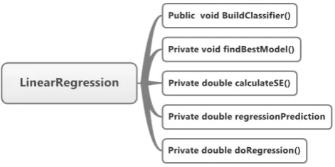
Figure 2 following a pseudo code division core of Linear Regression algorithm:
Figure2. Pseudo Code a Linear Regression Algorithm
Then to do the computation complexity of partially private_double_doRegression pseudo code is as follows:
...
private double [] doRegression(boolean [] selectedAttributes)
throws Exception {
if (b_Debug) { //O(1)
System.out.print("doRegression(");
for (int i = 0; i < selectedAttributes.length; i++)
{ //O(N)
System.out.print(" " + selectedAttributes[i]); } System.out.println(" )"); }
int numAttributes = 0;
for (int i = 0; i < selectedAttributes.length; i++) { //O(N)
if (selectedAttributes[i]) { //O(1)
numAttributes++; } }
Matrix independent = null, dependent = null;
if (numAttributes > 0) { //O(1)
independent = new
Matrix(m_TransformedData.numInstances(), numAttributes); dependent = new
Matrix(m_TransformedData.numInstances(), 1); for (int i = 0; i <
m_TransformedData.numInstances(); i ++) { //O(N) Instance inst = m_TransformedData.instance(i);
double sqrt_weight = Math.sqrt(inst.weight()); int column = 0;
for (int j = 0; j < m_TransformedData.numAttributes();
j++) { //O(N)
...
Figure 3. Some pseudo code Linear Regression calculated algorithm complexity.
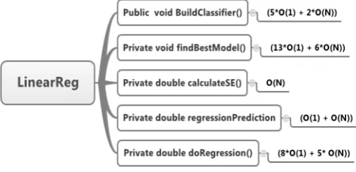
Figure 4. Analysis of Big-O complexity algorithm Linear Regression.
Then pseudo code of the core is obtained calculation of total Big-O as follows:
Table 1. Total Complexity Algorithm Linear Regression
Pseudo Code Complexity
buildClassifier (5*O(1) + 2*O(N))
findBestModel (13*O(1) + 6*O(N))
calculateSE O(N)
regressionPred (O(1) + O(N))
doRegression (8*O(1) + 5* O(N))
2) SMO Regression Algorithm
As for the distribution of pseudo code algorithm SMORegression core can be seen in Figure 5.
Figure 5. Pseudo Code SMORegression calculated algorithm complexity.
...
public double[] distributionForInstance(Instance inst) throws Exception {
if (!m_checksTurnedOff) { //O(1)
m_Missing.input(inst); m_Missing.batchFinished(); inst = m_Missing.output();}
if (m_NominalToBinary != null) { //O(1)
m_NominalToBinary.input(inst); m_NominalToBinary.batchFinished(); inst = m_NominalToBinary.output(); }
if (m_Filter != null) { //O(1)
m_Filter.input(inst); m_Filter.batchFinished(); inst = m_Filter.output();}
if (!m_fitLogisticModels) { //O(1)
double[] result = new double[inst.numClasses()]; for (int i = 0; i < inst.numClasses(); i++) {
for (int j=i+1;j< inst.numClasses();j++) { //O(N^2) if ((m_classifiers[i][j].m_alpha != null) ||
(m_classifiers[i][j].m_sparseWeights != null)) { double output = m_classifiers[i][j].SVMOutput(-1, inst);
if (output > 0) { //O(1)
result[j] += 1; } else result[i] += 1; ...
Figure 6. Some pseudo code SMORegression calculated algorithm complexity.
Figure 7. Analysis of Big-O complexity algorithm SMORegresion.
Then the pseudo code of the core is obtained calculation of Big-O as follows:
Table 2. Total Complexity Algorithm SMORegression
Pseudo Code Complexity
instanceInput ((6 * O(1) + O(N) + O(N2))
buildClassifier ((11*O(1) + 7 O(N) + O(N2))
doubleBias O(N2)
stringOutput ((3*O(1) + (N2))
3) Multilayer Perceptron Algorithm
In the multilayer perceptron algorithms are 6 main pseudo code used to generate the data output forecasting. When depicted in chart form are as follows:
Figure 8. Pseudo code Multilayer Perceptron Algorithm
The following is a portion of the pseudo code Multilayer Perceptron algorithm to calculate its complexity:
...
private Instances setClassType(Instances inst) throws Exception {
if (inst != null) { //O(1)
double min=Double.POSITIVE_INFINITY; double max=Double.NEGATIVE_INFINITY; double value;
m_attributeRanges=new double[inst.numAttributes()]; m_attributeBases=new double[inst.numAttributes()];
for (int noa = 0; noa < inst.numAttributes(); noa++) { //O(N)
min = Double.POSITIVE_INFINITY; max = Double.NEGATIVE_INFINITY;
for (int i=0; i < inst.numInstances();i++) { //O(N)
if (!inst.instance(i).isMissing(noa)) { //O(1)
value = inst.instance(i).value(noa);
if (value < min) { //O(1) min = value; }
if (value > max) { //O(1)
m_attributeRanges[noa] = (max - min) / 2; m_attributeBases[noa] = (max + min) / 2;
if (noa != inst.classIndex() && m_normalizeAttributes) { //O(1)
Figure 9. Some Pseudo code Multilayer Perceptron calculated algorithm complexity.
As for the calculation of the Big-O of 6 Multilayer Perceptron pseudo code is as follows:
Figure 10. Analysis of Complexity of Big-O Multilayer Perceptron algorithm.
Analysis of the complexity of the pseudo code above is as follows:
Table 3. Total Complexity MLP Algorithm
Pseudo Code Complexity
setClassType (8*O(1) + O(N*M) + O(N2)
public MLP (14*O(1) + O(N2))
setTrainingTime (10*O(1) + 3*O(N) + O(M*N))
caluculateOutput O(N)
CalculateError O(1) + O(M*N)
setOutput O(1) + O(N)
B. Running Time Analysis
This part discusses about the implementation of each algorithm into Weka application to test owned running time by every algorithm. The test is divided into seven steps; those are by cutting the data set with the number of 24, 36, 48, 60, 108, 224, & 448. Every test is divided into three times measurement of running time to make sure the accuracy of running time owned by each algorithm in handling several different data inputs. Here it is the table of measurement result that has been conducted. Time measurement is conducted by hour, minute, and second unit (00:00:00).
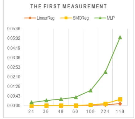
Table 4. The First Measurement
Sampel
Table 2. The Second Measurement
Sampel
Table 6. The Third Measurement
Sampel
Tables from 1-3 are the result toward all tests to data set that has been divided into several parts. MLP algorithm in the first, second, and third measurement had increasing running time every time it was tested with different number of data set. The more needed running time data is set by multi-layer perceptron algorithm, the bigger it could be compared to Linear Regression and SMORegression algorithms. It is similar to the second and third measurement result of Linear Regression and SMORegression (see figure 11-13 for running time comparison graphs every logarithm at the first time.
Figure 12. The Second Running Time Measurement Graph
Figure 13. The Third Running Time Measurement Graph
On the other hand, for Linear Regression and SMORegression algorithms from the first, second, and third (see table 1-3), running time needed is fluctuative. Globally, the increase of running time need for a great number of data set has significant influence to the use of great amount of running time (see figure 2 for running time comparison graph of the second measurement).
However, for both algorithm, they had running time which had slightly different toward the data with few numbers.
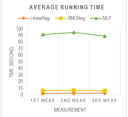
Table 7. Table of Running Time Average
Algorithm 1st Meas. 2nd Meas. 3rd Meas. LinearReg 2.28 2.57 2.57
SMOReg 4.42 4.28 3.85
MLP 85 88 83
In the form of graph, it can be drawn, as follow:
Figure 14. The Graph of Running Time Average
C. Comaprison Analysis of Complexity and Running Time This part is going to discuss about the analysis of each algorithm comparison after conducting the implementation to Weka application. Running time test was done by using the sample data achieved from Health Ministry of Yogyakarta Special Province; it was the occurrences of dengue fever from 1996-2006 consisting of 5 variables and data sample 948 data set. The test was divided into three steps, such as: sorting the data set and divide them into two fold started from 12, 24, 36, 48, 108, 224 & 448. Every test was divided into twice measurement of running time to make sure the accuracy of running time owned by each algorithm in handling several different data. Here it is the table of test result that had been conducted (see Table 1-3). From the result of the test based on algorithm complexity (Linear Regression, SMORegression & Multi-layer perceptron) and the number of the input data used as the sample (24, 36, 48, 60, 108, 224 & 448), the result gave different running time.
V. CONCLUSSION
Forecasting model needs process of data measurement mathematically. This study used 3 algorithms in conducting forecasting process with the input of time series data. To achieve a good forecasting result, it needs an algorithm concept that considered space complexity and complexity of time. The algorithms used were Linear Regression, SMORegression and Multilayer Perceptron. The calculation of algorithm used Big-O analysis, while to count time complexity used running time analysis from each algorithm. By looking at the result of those several experiments, it can be concluded that running time is significantly influenced by algorithm’s complexity and additional data set numbers that became the input.
Regression, SMORegression, and the last was Multilayer Perceptron.
VI. REFERENCES
[1] D. N. P. Murthy and K. C. Staib, “Forecasting maximum speed of aeroplanes — A case study in technology forecasting,” IEEE Trans. Syst. Man. Cybern., vol. SMC-14, no. 2, pp. 304–310, 1984.
[2] K. Huarng and T. H. K. Yu, “Ratio-based lengths of intervals to improve fuzzy time series forecasting,” IEEE Trans. Syst. Man, Cybern. Part B Cybern., vol. 36, no. 2, pp. 328–340, 2006. [3] H. Sen Yan and X. Tu, “Short-term sales forecasting with
change-point evaluation and pattern matching algorithms,”
Expert Syst. Appl., 2012.
[4] P. Cortez, M. Rocha, and J. Neves, “Evolving time series forecasting ARMA models,” J. Heuristics, vol. 10, pp. 415–429, 2004.
[5] S. Shukla, S. Kumar, and B. Verma, “A linear regression-based frequent itemset forecast algorithm for stream data,” 2009 Proceeding Int. Conf. Methods Model. Comput. Sci., pp. 1–4, Dec. 2009.
[6] L. Wang, L. Tan, C. Yu, and Z. Wu, “Study and Application of Non-Linear Time Series Prediction in Ground Source Heat Pump System,” no. 19005114009, pp. 3522–3525, 2012. [7] J. J. Hopfield, “Neural networks and physical systems with