Quantification of Axial Solids Mixing and Impacts of Internals in a Liquid-Solids Circulating Fluidized Bed Downer

(1)

Scholarship@Western

Electronic Thesis and Dissertation Repository

4-17-2014 12:00 AM

Quantification of Axial Solids Mixing and Impacts of Internals in a

Liquid-Solids Circulating Fluidized Bed Downer

Ha Doan

The University of Western Ontario

Supervisor Jesse Zhu

The University of Western Ontario

Graduate Program in Chemical and Biochemical Engineering

A thesis submitted in partial fulfillment of the requirements for the degree in Master of Engineering Science

Follow this and additional works at: https://ir.lib.uwo.ca/etd

Part of the Chemical Engineering Commons

Recommended Citation Recommended Citation

Doan, Ha, "Quantification of Axial Solids Mixing and Impacts of Internals in a Liquid-Solids Circulating Fluidized Bed Downer" (2014). Electronic Thesis and Dissertation Repository. 2029.

https://ir.lib.uwo.ca/etd/2029

This Dissertation/Thesis is brought to you for free and open access by Scholarship@Western. It has been accepted for inclusion in Electronic Thesis and Dissertation Repository by an authorized administrator of

(2)

(Thesis format: Monograph Article)

by

Ha Doan

Graduate Program in Chemical and Biochemical Engineering

A thesis submitted in partial fulfillment of the requirements for the degree of

Master of Engineering Science

The School of Graduate and Postdoctoral Studies The University of Western Ontario

London, Ontario, Canada

(3)

ii

Abstract

Liquid solids circulating fluidized beds have great potential to be utilized in many chemical

processes for their tremendous advantages. There are many studies about the riser but there

is not any information on the downer as yet. This research is devoted to study the axial

solids mixing in the downer. A new methodology was developed based on the concept of

ion-exchanging ability of resins and the residence time distribution measurement. Resin

particles were loaded with calcium ion as the tracer and Peclet number and the axial

dispersion coefficient were determined for each set of operating conditions. Different

designs of baffles were implemented in order to examine their effects on the axial solids

dispersion. The results show that the baffles reduce the mixing substantially and their

suppression effects increase with liquid velocity, except at very low liquid velocity where the

presence of the baffle increases the mixing. Among the three designs – louver, mesh, and

vertical plane, the louver has the most influence as it reduces the mixing coefficient by 60%

when Ul = 3.86Umf. Under the same conditions, the mesh and vertical plane reduce the

mixing coefficient by 46% and 32% respectively.

Keywords

Liquid-Solids Fluidization, Downer, Counter-Current, Axial Solids Mixing, Dispersion,

(4)

iii

I would like to express the deepest appreciation to my supervisor, Dr. Zhu who is

well-known for his knowledge as a researcher, and for his supportive attitude as a professor. He

has set a bright example of a successful academic professional. I did not have him in my

undergrad, and it is my honour to be his student now. Despite his busy schedule, my

supervisor always makes himself available for weekly meetings with students. I am grateful

for his time, for him always being smiling and positive, and giving me many insightful

counsels. Without his encouragement and guidance, this thesis would not have been

possible.

It is with immense gratitude that I acknowledge the support and help of my industrial partner,

Renix Inc. and its president, Ms. Christine Haas. Ms. Haas and her colleagues have provided

me many useful ideas and advices, and given me a chance to work in their facility and use

their lab equipments. I am indebted to the colleagues who had helped me develop my

methodology and repair the lab apparatus. I owe my deepest gratitude to Ms. Haas for her

financial and intellectual supports to my research. This opportunity is an invaluable

experience to me.

In addition, I would like to thank Dr. Gomaa for his valuable input which helped me find a

way to interpret my experimental data. I thank Mr. Wen and Mr. Li – the technicians in Dr.

Zhu's group, for their work getting the pilot scale unit ready. The financial support was

provided by the University of Western Ontario, Renix Inc., MITACS and the Ontario Centres

(5)

iv

List of Figures

Figure 1.1: Fluidized particles behave like liquid ... 2

Figure 2.1: Schematic diagram of a typical (G-)LSCFB system (Razzak et al., 2009) ... 7

Figure 2.2: Schematic diagram of liquid distributors in a LSCFB a) riser (Razzak et al., 2009)

b) downer ... 8

Figure 2.3: Variation of the axial liquid holdup distribution in the conventional and

circulating regimes for 0.405mm glass beads (Liang et al., 1997) ... 10

Figure 2.4: Circulation rate versus liquid velocity for three types of particles (Zheng et al.,

1999) ... 11

Figure 2.5: Determination of liquid transition velocity for the three types of particles (Zheng

et al., 1999) ... 12

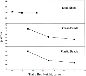
Figure 2.6: The effect of total solids inventory (expressed as the static bed height in the

storage vessel before the start of solids circulation) on the critical transition velocity for

plastic beads, glass bead I and steel shots (Zheng & Zhu, 2001) ... 13

Figure 2.7: Time required for all the particles to be entrained out of the bed, as a function of

liquid velocity for glass beads I and plastic beads (Zheng & Zhu, 2001) ... 14

Figure 2.8: Flow regime map for liquid-solid circulating fluidized bed (Zhu et al., 2000) .... 16

Figure 2.9: Variations of the solids circulation rate with the total liquid flowrate (Zheng et al.,

1999) ... 18

Figure 2.10: Variation of the axial solids holdup distribution with liquid velocity in the

circulating fluidization regime for glass beads and steel shots (Zhu et al., 2000) ... 19

Figure 2.11: Average solids holdup versus liquid velocity at different solids circulation rates

(10)

ix

all three types of particles (Zheng et al., 1999) ... 21

Figure 2.13: Variation of solids holdup with the primary and auxiliary liquid velocities

(Palani & Ramalingam, 2008) ... 21

Figure 2.14: Radial distribution of liquid velocity under Gs = 5 (a) and 10 (b) kg/m2s and

different liquid velocities for glass beads (Zheng & Zhu, 2003) ... 23

Figure 2.15: The radial distribution of the liquid velocity under different particle circulating

rates (Zheng & Zhu, 2003) ... 24

Figure 2.16: The radial distribution of solids holdup at four bed levels at (a) different

superficial liquid and (b) solids velocities for glass beads (Zhu et al., 2000) ... 25

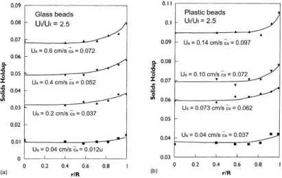
Figure 2.17: Comparison of the radial solids holdup profiles for glass beads and plastic beads

under the same cross-sectional average solids holdup ( ) at H = 0.8m (Zheng et al., 2002) ... 26

Figure 2.18: Radial profiles of solids holdup at the level H = 0.8m for different solids

flowrates for (a) glass beads and (b) plastic beads at the same normalized liquid velocity,

(Zheng et al., 2002) ... 27

Figure 2.19: The radial distributions of particle velocity at different superficial liquid

velocities for glass beads averaged axially over the riser (Roy et al., 1997) ... 29

Figure 2.20: Variation of superficial solid velocity with the superficial liquid velocities at

different auxiliary liquid velocities for glass beads (500 and 1290 μm) (Razzek et al., 2009)

... 30

Figure 2.21: Radial distribution of solids holdups for glass beads (500 and 1290 μm) at axial

location h = 2.02 m and Ul = 22.4 cm/s (Razzak et al., 2009) ... 31

Figure 2.22: Typical tracer concentration distribution profiles (Ul0 = 0.072 m/s, ε = 0.9, Gs =

7.5 kg2m-1s-1) (Chen et al., 2001) ... 32

(11)

x

Figure 2.25: Effects of superficial liquid velocity on liquid radial mixing (Chen et al., 2001)

... 34

Figure 2.26: Effects of solid holdup on liquid radial mixing (Chen et al., 2001) ... 35

Figure 2.27: Residence time distribution calculated from CARPT data (Ul = 20 cm/s; S/L =

0.10) (Roy & Dudukovic, 2001) ... 36

Figure 2.28: Pressure drop - velocity relationship (Couderc, 1985) ... 38

Figure 2.29: Bed height - velocity relationship (Yang, 2003) ... 38

Figure 2.30: (a) Pressure drop and (b) bed expansion of resin bed as a function of vessel

diameter. Water velocities (mm/s) 1) 0.5; 2) 1.2; 3) 1.9; 4) 5; 5) 6; 6) 9 (Nikitina et al., 1981)

... 39

Figure 2.31: Superficial velocity - bed voidage relationship (Chhabra, 2007) ... 40

Figure 2.32: Radial particle holdup distribution under different operating conditions and at

different bed sections for 0.405 mm glass beads. (●) Ul = 0.034 m/s, Us = 0; (∆) Ul = 0.078

m/s, Us = 0.0019 m/s; (◊) Ul = 0.078 m/s; Us = 0.0011m/s (Liang et al., 1997) ... 42

Figure 2.33: Effects of flow velocity on (a) the axial mixing coefficient and (b) the

Bodenstein number (Tong & Sun, 2001) ... 43

Figure 2.34: Axial mixing coefficient as a function of degree of bed expansion (Tong & Sun,

2001) ... 44

Figure 2.35: Effect of liquid viscosity on axial mixing coefficient: (ᴏ) NFBA-S / water; (●)

NFBA-S / 10%(v/v) glycerol; (∆) NFBA-L / water; (▲) NFBA-L / 10%(v/v) glycerol; (□)

Streamline SP / water; (■) Streamline SP / 10% (v/v) glycerol (Tong & Sun, 2001) ... 45

Figure 2.36: Effect of distributors on the response of the liquid fluidized bed at different

(12)

xi

velocities (Asif et al., 1991) ... 48

Figure 2.38: Effect of column size on (a) axial mean solids velocity, (b) dispersion coefficients (Limtrakul et al., 2005) ... 49

Figure 2.39: Effect of distributor type on (a) axial mean solids velocity, (b) dispersion coefficients (Limtrakul et al., 2005) ... 50

Figure 2.40: Effect of superficial liquid velocity on (a) axial mean solids velocity, (b) dispersion coefficients (Limtrakul et al., 2005) ... 51

Figure 2.41: Effect of particle size at Ul/Umf = 1.7 (Ul = 7 cm/s for 0.003 m; Ul = 2.4 cm/s for 0.001 m) on (a) axial solids velocity and (b) dispersion coefficients (Limtrakul et al., 2005) 52 Figure 2.42: Effect of particle density at Ul/Umf = 1.7 (Ul = 7 cm/s for glass beads; Ul = 2.4 cm/s for acetate) on (a) axial solids velocity and (b) dispersion coefficients (Limtrakul et al., 2005) ... 53

Figure 3.1: 5-cm column apparatus ... 56

Figure 3.2: Liquid distributor used in lab scale ... 57

Figure 3.3: Schematic diagram of the downer ... 58

Figure 3.4: Loading Ca2+ onto resin ... 59

Figure 3.5: Calibration curve for S 1668 resins ... 64

Figure 3.6: Calibration curve 1 for SGC 650 resins ... 65

Figure 3.7: Calibration curve 2 for SGC 650 resins ... 66

Figure 4.1: Comparing RTD at different solids velocities ... 70

Figure 4.2: Comparing RTD when bed height changes ... 71

(13)

xii

Figure 5.2: Mesh baffle ... 76

Figure 5.3: Vertical plane ... 77

Figure 5.4: Positions of the baffles in the downer ... 78

Figure 6.1: Residence time distribution graph ... 79

Figure 6.2: Illustration of the phosphorescent tracer method (Wei & Zhu, 1996) ... 81

Figure 6.3: Particle velocity measurement by using two-fiber sensor (Nieuwland et al., 1996) ... 82

Figure 6.4: RTD graphs in baffle-free setup at Ul = 1.45Umf ... 86

Figure 6.5: RTD graphs in louver baffle setup at Ul = 1.45Umf ... 87

Figure 6.6: RTD graphs in mesh baffle setup at Ul = 1.45Umf ... 87

Figure 6.7: RTD graphs in vertical baffle setup at Ul = 1.45Umf ... 87

Figure 6.9: RTD graphs in louver baffle setup at Ul = 2.66Umf ... 89

Figure 6.10: RTD graphs in mesh baffle setup at Ul = 2.66Umf ... 90

Figure 6.11: RTD graphs in vertical plane baffle setup at Ul = 2.66Umf ... 90

Figure 6.13: RTD graphs in louver-baffled setup at Ul = 3.86Umf ... 92

Figure 6.14: RTD graphs in mesh-baffled setup at Ul = 3.86Umf ... 92

Figure 6.15: RTD graphs in vertical plane setup at Ul = 3.86Umf ... 93

(14)

xiii

(15)

xiv

List of Appendices

Appendix A-1: Maximum capacity of SGC 650 resins for calcium ... 105

Appendix A-2: Maximum capacity of S 1668 resins for calcium ... 107

Appendix A-3: Calculate mass rate of solids circulation ... 108

Appendix A-4: Mole ratio between sodium and calcium in a sample desorption ... 109

Appendix A-5: Calibration curve for S 1668 resins ... 110

Appendix A-6: Calibration curve for SGC 650 resins ... 111

Appendix A-7: Verification of calibration curve ... 113

Appendix B-1: Data for lab-scale run 1 ... 114

Appendix B-2: Data for lab scale run 2 ... 117

Appendix C-1: Data for the baffle-free trial at Ul = 1.45Umf ... 126

Appendix C-2: Data for the louver trial at Ul = 1.45Umf ... 130

Appendix C-3: Data for the mesh trial at Ul = 1.45Umf ... 133

Appendix C-4: Data for the vertical plane trial at Ul = 1.45Umf ... 136

Appendix C-5: Data for the baffle-free trial at Ul = 2.66Umf (Run #1) ... 139

Appendix C-6: Data for the baffle-free trial at Ul = 2.66Umf (Run #2) ... 142

(16)

xv

Appendix C-9: Data for the vertical plane trial at Ul = 2.66Umf ... 151

Appendix C-10: Data for the baffle-free trial at Ul = 3.86Umf ... 154

Appendix C-11: Data for the louver trial at Ul = 3.86Umf ... 157

Appendix C-12: Data for the mesh trial at Ul = 3.86Umf ... 160

(17)

Chapter 1

1

Introduction

Fluidization is a process that involves contact of suspended solid phase with liquid and/or

gas phase. The technology has been utilized in many various fields and becomes more

and more important from industrial point of view.

1.1 First Description of Fluidization

When a bed of solid particles comes in contact with and is suspended in an upward fluid

flow, the solid bed is said to be in fluidization and the fluid is called fluidizing fluid.

Fluidizing fluid could be either liquid, or gas, or combination of both. The reason for the

name fluidization is that the solids bed gains a number of properties of liquid:

 Surface of a fluidized bed always maintains horizontal even if the bed is

positioned on an inclined plane.

 Solids can be poured out of the vessel through an opening without requiring any

mechanical device.

 A fluidized unit also exhibits a static pressure head due to gravity, given by

, where is density of the bed.

 When a number of units are connected, particles in the one with higher bed level

will flow to the more shallow one until the bed levels are the same, in order to

equalize their static pressure heads.

 If the bed is constituted of two types of particles with different densities, the layer

of the lighter particles floats on top while layer of the denser particles sinks at the

(18)

Figure 1.1: Fluidized particles behave like liquid

Depending on the phase of fluidizing fluid, fluidization is classified into three types:

gas-solids, liquid-gas-solids, and three phase gas-liquid-solids. Gas-solids was the first form of

this technology, born in 1920s and found its first application in coal gasification by

Winkler. The first large scale implementation was in 1940s in fluid catalytic cracking

process (Anon, 1962). In 1950s was the emergence of liquid-solids fluidization. Over

the decades, intensive studies have been done to understand the hydrodynamic

behaviours of both gas-solids and liquid-solids fluidization systems due to their great

advantages:

 Efficient interphase contact

 High mass transfer rate

 Even distribution of temperature

 Easy handling of large solids quantity

In some applications, particles lose their capacity over time as the process proceeds. For

instance, solid catalysts become deactivated in metallurgical or petrochemical operations,

or solid adsorbents are fully loaded in adsorption processes. As a result, they require a

new batch of particles. In the past, to accommodate this demand, a number of vessels

were built. When solids in a vessel became inactive after a period of time, a new unit

took the position to continue the operation while the former one was being regenerated.

Even though this method could provide a continuous process, batch operation still poses a

(19)

 Possible inconsistency in product grades from batch to batch

 High labour cost

 Low throughput

 Low productivity

 High back-mixing of phases

These limitations motivated the invention of an uninterrupted system: circulating

fluidized beds. The inception of liquid – solids circulating fluidization in 1960s (Zhu et

al., 2000) has become useful and been implemented in many areas. Some of them

employ circulating fluidized units because their applications constantly require fresh

particles like aforementioned examples. They need to have a continuous system to

remove inactive solids and feed in the regenerated ones. Some others utilize this

circulating fluidized bed technology because they operate liquid feed at high flowrate.

The particles used are light and small, thus get entrained out of the column.

Consequently, it is essential to keep feeding the particles into the column. With the

advantages of the uninterrupted operation, liquid-solids circulating fluidization is widely

used in many fields such as in food processing, water treatment, and metallurgical

industries.

One example is the application of a liquid solids circulating fluidized bed (LSCFB) to

recover proteins from waste streams which contains low protein concentration. The

adsorption and desorption of proteins are accomplished separately in the two parallel

columns: downer and riser, respectively. The solids used are ion-exchange resins which

are circulated between these two columns. The feed broth is introduced from the bottom

of the downer. The protein in the liquid phase is adsorbed onto the resins. While the

de-proteinized liquid stream is discarded from the top of the downer, the loaded particles

exit the bottom of the downer to enter the riser. Desorption buffer is fed via a liquid

distributor placed at the bottom of the riser, and carries the resins upward while

desorbing protein out of the resins. After releasing the proteins, the resins are considered

fresh, or regenerated. The regenerated particles are then separated from the buffer

(20)

circulation cycle (Zhu et al., 2000; Zheng et al., 2002). (More details about system

configurations can be found in Section 2.1)

The performance of an LSCFB relies on the two key factors: the chemistry aspect and the

hydrodynamics aspect. The chemistry varies from application to application since it

depends on the type of solids used, the treating liquid stream, and their reaction kinetics.

As a result, this aspect cannot be generalized but needs to be considered for each

individual case. In contrast, the hydrodynamics knowledge can be applied into design

and scale-up in most cases. Even though this is an area of research since 1990s and

becomes more and more popular over the years, some information is still incomplete.

One of the missing pieces on this hydrodynamics picture is the longitudinal dispersion of

solid phase in the downer.

1.2 Objectives

In order to properly design and scale up a LSCFB, it is important to understand the

hydrodynamics behaviour of the system, such as phase holdups and their distributions,

flow patterns and mixing levels of each phase (Limtrakul et al., 2005). A lot of studies

have been reported for the riser exploring all the areas mentioned above. However, there

is absolutely no available data on the downer. Often the fluid dynamics in the downer is

presumed to be similar to conventional fluidized beds where there is no net flow of solid

phase. This might be premature assumption for the downer at least about the mixing

levels. In conventional fluidized beds, there is only upward flow of liquid whereas in

downer the liquid and solids flow counter-currently, so that a conventional fluidized bed

and a downer bed are incomparable. In other words, mixing levels in conventional

fluidized beds cannot be representative for ones in downer. To avoid the same

presumption, this project is designed to investigate mixing level of solid phase in the

axial direction in the purpose of providing some insight about what is happening within

the downer bed.

To conduct this study, a new method for particle tracking is developed since all other

tracking techniques for solid phase are either inapplicable or unavailable. The new

(21)

method at this point because no data is reported in this area as yet. However,

demonstration of the method can be performed within the scope of this study.

Longitudinal solids dispersion, also termed as back-mixing, is an important parameter to

evaluate performance of a fluidized bed. It describes the random motion of particles in

the axial direction and is driven by the diffusion force. In mixers, this type of motion is

desirable since it promotes mixing. However, in fluidized beds, longitudinal dispersion

of solids is better to be constrained. Large dispersion is an indication of broad

distribution of solids residence time. On one side, some particles exit the system earlier

than the expected time. In other words, the contact time between liquid and solid phases

is not long enough, leading to part of their capacity is unused. On the other side, some

particles exit the system much later than the designed contact time. This may cause two

problems. One is if the process involves catalysts or adsorbents that are heat-sensitive

and the reaction is exothermic, extended residence time may cause the damage to the

solid particles. The other is when the catalysts are deactivated or when the adsorbents are

fully adsorbed, their extra time residing in the bed does not results in a higher production

but only means process delay. For these reasons, for the best interest, axial solids mixing

should be minimized in the interest of obtaining the best performance.

Axial mixing of phases is often expressed as axial mixing coefficient, or Peclet number.

In an ideal case where there is absolutely no axial dispersion, the particles exit a column

in exact order as they have entered, the mixing coefficient would be zero and the Peclet

number is infinity. The increasing of the mixing coefficient, or the decreasing of Peclet

value indicates the distribution of particles is getting broader and the state of the fluidized

bed is further away from the ideal plug flow. There are many factors effecting

back-mixing of solids including but not limited to particle-particle collision, particle-wall

collision, turbulence due to liquid flow, also not perfectly vertical column setup,

non-ideal liquid distributor. The former three are infeasible to avoid as they are nature of

phase interaction; the latter two are possible to be improved. Nevertheless, making an

ideal distributor is extremely challenging because it has to provide equivalent hydraulic,

which means equivalent flowrate, equivalent time of passage and equivalent pressure

(22)

limited. To achieve the goal of restricting axial solids mixing, one could attempt to make

an ideal distributor facing those challenges and risking patent violation issues. In the

same purpose, this project demonstrates an alternative to constrain the random motion of

particles by inserting internals inside the downer fluidized bed. Different designs of

(23)

Chapter 2

2

Literature Review

In this chapter available data on the liquid-solids fluidization will be presented. The first

sections will cover the circulating fluidization hydrodynamics since the project is aimed

to study the downer of a liquid-solids circulation system. The later sections cover the

conventional fluidization hydrodynamics because no data is available for the downer as

yet, and downer is in the same fluidization regime as conventional beds. The literature

review for the circulating systems and the conventional systems are categorized into three

topics: axial profiles, radial profiles and phase mixing. The focus of this project is on

solids phase mixing, not liquid mixing or the axial and radial profiles, but all of them are

essential to understand the dynamic behaviours of a particular system, therefore the

discussion will be on all those topics.

2.1 LSCFB System Details

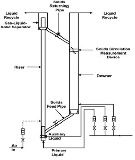
Figure 2.1 shows the schematic diagram of a typical (G-)LSCFB system.

(24)

The setup consists of two main parallel cylindrical vessels called riser and downer. The

processes taking place in these two reactors are often the reverse of each other, either

adsorption / desorption processes or reaction / regeneration processes. Therefore, they

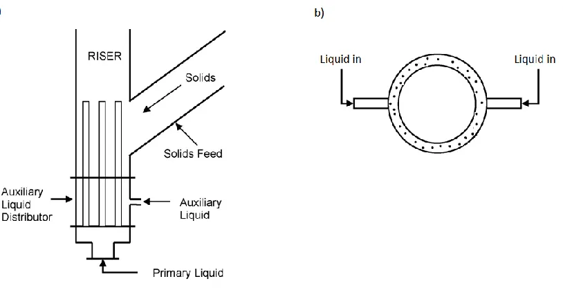
are fluidized by two different fluidizing liquids. Liquid injected into the riser is divided

into two streams: primary liquid and auxiliary liquid. There is distributor for each

stream. The main liquid distributor is made of one or multiple stainless steel tubes,

depending on the size of the vessel itself and the second liquid distributor is a porous

plate. Both are placed at the base of the riser (Figure 2.2a). There is also a distributor at

the conical bottom of the downer, which is a ring shape with multi-openings at different

locations and in different angles (Figure 2.2b).

Figure 2.2: Schematic diagram of liquid distributors in a LSCFB a) riser (Razzak et

al., 2009) b) downer

Particles are carried upward in the riser by conjunction of primary and auxiliary liquids.

The existence of the auxiliary stream is to mobilize the solids as they exit the feeding

pipe. In feeding pipe and returning pipe, solids travel like a packed bed. As they flow

down from the feeding pipe, they come in contact with the secondary liquid, and are

loosened up. The auxiliary stream works as a non-mechanical device to facilitate

particles to enter the riser, therefore controls how much or how fast solids entrance is.

(25)

liquid streams, solids circulation and total liquid velocity for the riser can be obtained

independently.

Both solids and liquid phase flow upward in the riser, and enter the liquid-solids

separator. The liquid-solids separator has conical bottom which allows solids to settle

and form a packed bed more easily while the liquid floats on top and exits via the liquid

outlet. The solids then return to the downer, passing through a solids circulation

measurement device. The device is positioned slightly below the returning pipe, and is a

vertical plate. It is divided by halves and equipped with two half butterfly valves at the

ends of the plate. To measure solids circulation rate, these two butterfly valves are

flipped to opposite direction for a short time interval, about a minute. As the top valve

blocks one side, then particles come to the other side only; the lower valve blocks that

side and captures the particles. By measuring the solids accumulation and knowing the

time taken, solids circulation rate can be calculated.

Particles enter the downer from the top and travel counter-currently to the liquid flow

which is upward. The downer has much higher solids concentration compared to the

riser because they are in different fluidization regimes. Their fluidization regimes will be

discussed in the following section of this chapter.

2.2 Fluidization Regimes

Fluidization of liquid-solids beds is controlled by superficial velocity of liquid. When

liquid velocity is low, the solid particles remain static, and they are considered in the

fixed state. When the fluid flowrate is high enough, the bed height starts to rise, and each

individual particle becomes suspended in the fluid. The bed is now considered in the

conventional fluidization regime. The value of liquid velocity that demarcates these two

states is called the minimum fluidization velocity, Umf, and can be calculated using Ergun

equation:

(26)

In both regimes, a clear boundary between the dense phase and freeboard phase is

observed. When the liquid velocity is increasing, the dense phase continues to expand.

Because the particles occupy a larger bed volume, the solids concentration becomes

lower. With further increase of liquid flow, the boundary between the two phases

becomes unclear. At sufficiently high liquid velocity, some particles start to get

entrained out of the column, suggesting the transition of fluidized beds from the

conventional regime to the circulating regime.

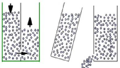
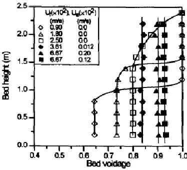
Figure 2.3 depicts dense phase, freeboard phase, and how dense phase expands with

liquid velocity increase. Looking at the two curves whose velocities are the lowest (Ul =

0.90 and 1.80 cm/s), which are the farthest left, all solids settle at the bottom of column.

In this dense phase, it is noted that the voidage is the same at all axial locations. Above

the dense phase, the voidage is 1.0, it means there is no solids in the higher region –

freeboard phase. When liquid velocity increases to 2.50 cm/s, the dense phase expands.

There is a dense zone up to bed height of 1.5 m, then dilute phase above that point. There

is no longer a clear boundary between dense phase and freeboard. At liquid velocity of

3.61 cm/s or higher, it can be seen from the legend box that Us is now above zero,

indicating the formation of solids circulation. The bed is in the circulating regime, and

there is only dilute zone. Bed voidage is constant along the bed height.

Figure 2.3: Variation of the axial liquid holdup distribution in the conventional and

(27)

The critical transition velocity

The point where particles start to get entrained out of the bed is termed as critical

transition velocity, Ucr. Liang et al. (1997) established a way to determine this value by

decreasing liquid velocity to the point where solids circulation stops and defined this

point as Ucr. It is confirmed that the critical transition velocity and the transition state are

affected by particle density. Shown in Figure 2.4, with increasing particle density, the

value of Ucr is higher and the transition becomes gradual. For example, for plastic beads

whose density is very low, solids circulation is formed at 0.01 m/s and the transition is

sharp, almost at a single liquid velocity. Contrarily, for steel shots, which are very heavy

particles, the transition starts much later at 0.21 m/s, and the range of liquid velocity for

transition is widened.

Figure 2.4: Circulation rate versus liquid velocity for three types of particles (Zheng

et al., 1999)

Zheng et al. (1999) further found the relation of transition velocity with particle terminal

velocity. Figure 2.5 shows that solids circulation stops as normalized liquid velocity

Ul/Ut approaches values between 1.0 and 1.1 for all 3 types of particles. That means

fluidization enters the circulating regime at transition velocity of equal or slightly higher

than the terminal velocity of particles. This information is quite appreciable for system

operation since solids terminal velocity can be calculated mathematically, and so the

(28)

Figure 2.5: Determination of liquid transition velocity for the three types of particles

(Zheng et al., 1999)

However, the critical transition velocity is found to be system operation dependent.

Zheng and Zhu (2001) reported this lower boundary limit of circulating regime varies

with the total solids inventory, which certainly affects the system pressure balance and

the pressure difference across the solids feeding pipe particularly. When the bed height in

the solids storage is increased, the pressure head at the base of the downer becomes

higher, leading to the pressure difference across the non-mechanical valve is also higher.

In turn, solids are fed to the riser faster. In other words, solids circulation increases at the

same liquid velocities. It also means the same solids circulation rate can be achieved at

lower liquid velocities when solids inventory is higher. Therefore, in identifying the

critical transition velocity by reducing liquid velocity until the solids velocity reaches

(29)

Figure 2.6: The effect of total solids inventory (expressed as the static bed height in

the storage vessel before the start of solids circulation) on the critical transition

velocity for plastic beads, glass bead I and steel shots (Zheng & Zhu, 2001)

The authors also noted how the critical transition velocity at first decreases drastically,

then gradually when static bed height is increased. It is explained that when back

pressure is high enough, the pressure distribution within the system has less influence on

the transition velocity. This observation is more discernible in the case with lighter

particles. The change in the transition velocity is hardly recognized in the steel shots

system over the experimental range due to equipment limitation and high particle density.

Overall, it is suggested to have a very high solids inventory when determining the value

of the critical transition velocity in order to minimize the system configuration

dependency and have the most accurate result.

The onset velocity

Since the critical transition velocity is intrinsically system dependent, it poses uncertainty

in defining the lower boundary of circulating fluidization regime. Zheng and Zhu (2001)

(30)

method is to measure how long it takes to empty a solids bed when there is no solids feed

from the storage vessel at a particular fluidizing liquid velocity. When the liquid flowrate

is slow, the time it takes for all particles to entrain out of the bed is very long. When the

flowrate is higher, this process certainly takes less time. Zheng and Zhu observed that

with increasing liquid velocity, the bed-emptying time is shortened drastically. Yet, to a

certain point, further increase of liquid flow does not affect the emptying time as much.

This turning point is marked as the onset velocity, Ucf. This phenomena is presented

graphically in Figure 2.7. A steep line and a flatter line are seen and their intersection

locates the onset velocity. The location of the onset velocity does not change with the

initial bed volumes (486 and 811 cm3). In addition, the method does not involve solids

feeding. Therefore it is independent of solids storage volume and the configuration of the

feeding system.

Figure 2.7: Time required for all the particles to be entrained out of the bed, as a

function of liquid velocity for glass beads I and plastic beads (Zheng & Zhu, 2001)

Onset velocity versus critical transition velocity comparison

Table 1 shows the determined onset velocity and critical transition velocity for 4 types of

particles, including their terminal velocity. Recalled from the previous discussion, the

(31)

is high enough, this influence becomes less noticeable. That means the transition

velocity determination is less varying when the storage static bed height is large. For the

reason, the values presented in Table 1 are obtained under the highest bed height tested

Lo = 1.5 m.

Table 2.1: The onset and critical transition velocities for different particles (Zheng

& Zhu, 2001)

The results show both the onset and the critical transition velocities are higher than the

terminal velocity. It is reasonable since system has to operate at a liquid velocity higher

than the particle terminal velocity in order to transport particles out of the bed. The onset

is slightly lower than the critical velocity. Another note should be taken from the table

above is that the ratios Ucf/Ut for various particle types are all about 1.1. Since Ucf is not

affected by the geometrical conditions, it only depends on liquid and solids properties.

Zheng and Zhu (2001) suggested a correlation for Ucf as following:

where a is a function of liquid properties such as density and viscosity. Based on the

experimental results, for tap water a is approximately 1.1 when operation is at room

temperature.

To summarize, the critical velocity is the true value defining the transition from the

conventional to the circulating fluidization regime and it varies with the operation setup.

The onset velocity is the lowest Ucr and a convenient way to demarcate the two regimes

independently from the geometry of the system. Therefore, it is accepted as the absolute

(32)

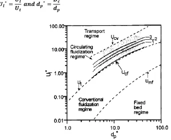
Beyond the circulating fluidization regime is the transport/hydraulic regime. In this state,

the particles continue to be carried out of the column. The only distinction between the

circulating and the transport regime is the radial profile of solids holdup. In the

circulating regime, solids concentration is higher near the wall and more dilute at the

center; whereas in the transport regime, the radial solids holdup is uniform. The

transition velocity between the two regimes is defined as Ucv (Liang et al., 1997). It is

expected that Ucv would increase with solids circulation rate. When solids feed is fast,

solids concentration is higher, leading to a solids concentration profile that is more

non-uniform. As the result, it requires higher liquid input to "smooth" out this non-uniformity

of radial solids profile, and enters the transport regime.

All fluidization regimes and transition velocities are summarized and presented in the

regime map below. The axis are dimensionless liquid velocity and dimensionless

particle size

Figure 2.8: Flow regime map for liquid-solid circulating fluidized bed (Zhu et al.,

(33)

2.3 Liquid-Solid Circulating Fluidized Bed Riser

The riser of a LSCFB system is fluidized by a fast flowing liquid. The liquid velocity is

so high that it transports the solid particles out of the bed. The riser bed is in co-current

circulating fluidization state.

2.3.1 Axial Hydrodynamic Behaviour

The Initial Zone and the Developed Zone

As liquid velocity reaches the transition velocity, Ucr, the fluidized bed enters the

circulating regime. In this regime, there exists two zones: initial zone and developed

zone. In the initial zone, solids circulation rate increases substantially with increase of

total liquid velocity. Shown in Figure 2.9 below, the initial zone occurs in a very narrow

range of liquid velocity to a point of being negligible for light particles such as plastic

beads, but this range of liquid velocity becomes much widened as particle density

increases. In the developed zone, the increase of liquid velocity affects solids circulation

insignificantly for all particle densities. The liquid velocity that marks the transition from

the initial circulating fluidized zone to the fully developed zone is the critical liquid

velocity, Ulc (Palani & Ramalingam., 2008; Natarajan et al., 2007). Natarajan et al.

(2007) proposed its value is 1.3 times the particle terminal velocity. It is suggested to

operate a system at a lower liquid velocity than the critical velocity if high solids holdup

is desired. Oppositely, liquid velocity should be higher than Ucr if a dilute phase and high

(34)

Figure 2.9: Variations of the solids circulation rate with the total liquid flowrate

(Zheng et al., 1999)

For heavy particles, such as steel shots with density of 7000 kg/m3, the axial profile of

solids holdup is not uniform in the initial circulation zone when the liquid velocity is low

(Ul = 26 and 28 cm/s). Recall from Table 1 the critical transition velocity of steel shots is

24.84 cm/s. When liquid velocity is 26 or 28 cm/s (Figure 2.10), it is the beginning of

circulating fluidization. Solids entering the riser from the bottom are usually in

downward or horizontal direction, they have zero or negative velocity. They need some

time to accelerate; therefore solids holdup tends to be denser at the lower region than at

the higher region. When particle density is low, the accelerating time is very short but for

high density particles, their development is much slower, leading to longer accelerating

distance. With further increase of liquid velocity (Ul = 35 cm/s), fluidization enters the

developed zone and axial solids holdup is uniform throughout the column. For glass

beads, the system is in developed circulating fluidization zone at lower liquid velocity (10

(35)

Figure 2.10: Variation of the axial solids holdup distribution with liquid velocity in

the circulating fluidization regime for glass beads and steel shots (Zhu et al., 2000)

The initial zone and developed zone are distinct from one another not only in terms of the

variation of solids circulation (Figure 2.9) and axial solids distribution (Figure 2.10) with

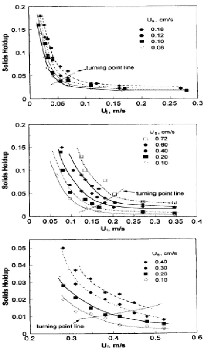
change in liquid velocity, but also in term of average solids holdup. Figure 2.11

expresses how average solids holdup changes with total liquid velocity. The graphs show

different trends in the initial zone and developed zone. In the initial zone, the graphs are

very steeply downward for all three types of particles. The indication is that the average

solids holdup decreases drastically with increasing liquid velocity. This is because when

liquid flows fast, it carries solids out of the riser quickly. Consequently, solids residence

time is shortened, leading to less solids holdup. In contrast, the graphs show a plateau in

the developed zone. Solids holdup is reduced much more slowly in this zone. It can be

explained that at a certain point, the increase in liquid velocity does not affect solids

circulation rate, as seen in Figure 2.9. As the result, the decrease of average solids

holdup with liquid velocity becomes less noticeable. Also seen in Figure 2.11, when

solids circulation rate increases, more solids are fed into the column, hence solids holdup

(36)

Figure 2.11: Average solids holdup versus liquid velocity at different solids

circulation rates for (a) plastic beads, (b) glass beads, and (c) steel shots (Zheng et

al., 1999)

Another note taken from Figure 2.11 is that particles density has strong influence on

hydrodynamic behaviour in the initial and developed zone. For light particle (plastic

beads), solids holdup decreases quickly, from 0.15 to 0.05. For heavy particle (steel

shots), solids holdup decreases very slowly, from 0.04 to 0.01. Yet, when fluidization is

fully developed, solids holdup profile reaches the same value 0.01 for all three types of

particles if under the same solids circulation rate (Figure 2.12). Therefore,

hydrodynamics in the initial zone varies by particle density, sharp for light particles and

gradual for heavy particles. When it reaches full development, they all experience the

(37)

Figure 2.12: Average solids holdup versus liquid velocity at a given solids circulation

rate for all three types of particles (Zheng et al., 1999)

Variation of Solids Holdups with Liquid Velocities

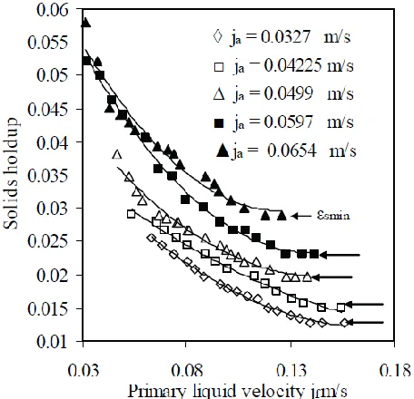
Palani and Ramalingam (2008) conducted their experiments to relate solids holdup with liquid velocity. In their study, they used sand whose diameter is 550 μm and the result is shown in the graph below.

Figure 2.13: Variation of solids holdup with the primary and auxiliary liquid

(38)

It is seen that when fixing the auxiliary velocity and turning up the primary liquid

velocity, the solids holdup is decreased. When liquid is fed into the riser at a faster rate,

more particles are transported out, as a result, less particles are present inside the column.

Oppositely, if one looks vertically, across the drawn lines, the data points show how

solids holdup in the riser changes when the primary is constant and the auxiliary varies.

The solids holdup increases with the auxiliary velocity. This can be explained by the

function of the auxiliary stream to loosen up the plug flow in the returning pipe and to

mobilize the particles as they are emerging the flow in the unit. In conclusion, the main

liquid stream is to carry the solid particles upward and entrain them out of the riser;

whereas the secondary stream is to aid the solids feeding system. Therefore the solids

holdup in the riser increases with increase of the secondary stream but with decrease of

the main stream. The knowledge of this variation is definitely beneficial for optimizing

operating conditions.

2.3.2 Radial Hydrodynamic Behaviour in LSCFB

Unlike conventional fluidization regime and transport regime, radial profiles of liquid

velocity, solids velocity and solids holdup in liquid - solids circulating regime are

non-uniform. The non-uniformity may have negative effects on the productivity of fluidized

beds since it causes uneven interphase contact. Therefore, understanding radial flow

structure is crucial to design reactors and to optimize processes.

Radial Distribution of Liquid Velocity

The radial distribution of liquid velocity presented in Figure 2.14 is at solids circulation

flux of 5 and 10 kg/m2s and different liquid velocities. The liquid velocity profile under

conventional fluidization regime, which means no solids circulation Gs = 0, is also

(39)

Figure 2.14: Radial distribution of liquid velocity under Gs = 5 (a) and 10 (b) kg/m2s

and different liquid velocities for glass beads (Zheng & Zhu, 2003)

When fluidization is in the conventional regime, the radial profile of liquid velocity is

uniform. The profile becomes non-uniform once solids circulation starts. Higher liquid

velocity occurs at the center (r/R = 0) and lower velocity is near the wall (r/R = 1.0).

This non-uniformity increases when liquid flows faster. For example, when Gs = 10

kg/m2s, graph is steeper when liquid velocity changes from 10 to 15 cm/s. With further

increase of liquid velocity (Ul = 28 cm/s), the graph flattens out, indicating the transition

from the circulating regime to the transport regime. In the dilute transport regime, solids

concentration is very low, thus the impact of solids presence on liquid profile is small. In

addition, when liquid velocity is quite high, liquid profile tends to distribute more

(40)

The effect of change in solids circulation on liquid velocity profile is also studied by

Zheng and Zhu (2003). At a fixed liquid velocity (Ul = 15 cm/s), the radial distribution

graph is steeper, means more non-uniformity, as solids circulation flux increases. A

possible explanation for this phenomenon is that when more solids are fed into the riser,

solids accumulation near the wall is greater than at the center. To accommodate this

variation, liquid flows more slowly near the wall than at the center.

Figure 2.15: The radial distribution of the liquid velocity under different particle

circulating rates (Zheng & Zhu, 2003)

Radial Solids Holdup Distribution

A typical radial distribution of solids holdup is plotted in Figure 2.16. It is seen that the

profile is not uniform. The solids concentration is higher at the wall (r/R = 1) than at the

center (r/R = 0). Measurements were done at 4 different heights along the riser: one in

the lower region (h = 0.3m), two at the middle region (h = 0.8 and 1.2 m) and one at the

upper region (h = 1.7 m). The data points at the same radial position are very close to

each other. It again proves that in liquid - solids circulating fluidization, the axial solids

(41)

Figure 2.16: The radial distribution of solids holdup at four bed levels at (a)

different superficial liquid and (b) solids velocities for glass beads (Zhu et al., 2000)

With an increase in liquid velocity from Ul = 10 to Ul = 14 cm/s (Figure 2.16a), the graph

gets steeper near the wall, indicating an increase in non-uniformity. As a natural

phenomenon, liquid flowing in a cylindrical pipe tends to flow faster at the center than at

the wall due to wall friction. Faster moving fluid at the center carries solids out more,

consequently makes solids holdup less at the core. When liquid velocity increases further

to 28 or 42 cm/s, the graphs flatten out. In other words, solids holdup is distributed

uniformly in the radial direction, indicating the transition to the transport regime. In

addition, a liquid velocity increase shifts the graph down, means solids holdup is reduced

at all radial positions. When liquid travels fast inside the riser, it entrains solids more

quickly, hence shortens solids retention time. As the result, solids holdup is overall less

at high liquid flowrate.

In Figure 2.16b, liquid velocity is fixed while solids velocity varies. It shows that when

solids circulation rate, which is expressed as solids velocity, increases, average solids

(42)

unchanged, the more solids are fed, the more solids are present in the column. Therefore,

solids holdup increases. In a denser zone, solids tend to accumulate at the wall even

more, leading to the difference in solids concentration at the wall and centre is widened.

This explains how the non-uniformity increases with solids velocity.

Non-uniformity in radial distribution of solids holdup is also affected by particle density.

The statement is demonstrated in the Figure 2.17 where the radial profiles of solids

holdup for glass beads and plastic beads are plotted. The two types of particles have

similar size and are fluidized in operating conditions that give the same average solids

holdup ( . The profiles for each type of particles under two different operating conditions almost coincide with each other when the cross-sectional average

solids holdups are the same. Comparing the profiles of the two particles types, the lighter

particles (plastic beads) have more uniform distribution, giving flatter parabolic curve.

This phenomenon is possibly due to the lower value of the ratio . When the density ratio is large, solids have a tendency to agglomerate at the wall more. For example in gas

- solids fluidization, the density ratio is very high, and significant cluster agglomeration is

seen. A conclusion that may be drawn here is that high density ratio worsens uniformity in radial solids holdup distribution.

Figure 2.17: Comparison of the radial solids holdup profiles for glass beads and

(43)

In the previous case, the average solids holdup is kept constant. In the following study,

the normalized liquid velocity remains unchanged and the impact of particle density on

solids holdup is investigated. Figure 2.18 presents radial profiles of solids holdup for

glass beads and plastic beads under different solids circulation rates. For light particles

(plastic beads), small increment of solids velocity, from 0.04 to 0.14 cm/s, increases

average solids holdup substantially. In contrary, for heavier particle an increment of

solids velocity, for instance from 0.04 to 0.2 cm/s, does not affect average solids

concentration greatly. Additionally, at the same solids velocity , plastic beads experience more solids holdup non-uniformity compared glass beads.

Again, this is because a higher concentration of solids always leads to more uneven

distribution.

Figure 2.18: Radial profiles of solids holdup at the level H = 0.8m for different solids

flowrates for (a) glass beads and (b) plastic beads at the same normalized liquid

(44)

Solids Acceleration

When solids enter the column from the returning pipe, they have velocity of zero or even

negative due to their direction either horizontal or downward at the entrance. They need

to be accelerated by the drag force that the liquid exerts on them. After this point, their

velocity is constant. Therefore there exist two regions: initial region, where particles

accelerate, located at the bottom of riser, and fully developed region, where particle

velocity is unchanged.

The length of the developing region, also called acceleration length, depends on liquid

and solids velocity and also density ratio. When liquid velocity is high, this length is

shortened because the drag force is higher. In opposite, an increase of solids circulation

rate makes this region extend longer since the same drag force supports a heavier mass.

Another factor impacting the acceleration length is the ratio ρs/ρl. The larger the ratio is,

the longer the length is. For example, in gas - solids fluidized beds, the density ratio ρs/ρg

is very high. For this reason, the developing region extends and could even takes up the

entire column, leading to non-uniformity in axial direction throughout the column in

gas-solids fluidization. For liquid - gas-solids fluidization, the density ratio ρs/ρl is much smaller,

especially for light particles for which the density ratio is close to unity. Consequently,

the developing region sometimes does not seem to exist.

Radial Distribution of Particle Velocity

There is limited study on radial distribution of particle velocity in liquid - solids fluidized

beds. Roy et al. (1997) employed large and dense particles (dp = 2.5 cm and ρs = 2500

kg/m3) to conduct their experiments measuring local solids velocity. Figure 2.19 shows

that increasing liquid velocity steepens the parabolic curve of particle velocity profile. It

was also found that there is no significant difference in local particle velocities at

different axial locations. Noticeably, the profile for particle velocity is more non-uniform

than for liquid velocity. Perhaps it is because the friction force between solids and wall is

higher than the one between liquid and wall. The friction force makes movement of

(45)

Figure 2.19: The radial distributions of particle velocity at different superficial

liquid velocities for glass beads averaged axially over the riser (Roy et al., 1997)

Particle Size Effects

A study of effects of particle size on hydrodynamics of LSCFB was done by Razzak

group (2009). They conducted experiments using two types of glass beads with

diameters of 500 μm (GB-500) and 1290 μm (GB-1290), both having the same density of

2500 kg/m3. Figure 2.20 shows the variation of solids circulation rate, expressed as

solids velocity, with the change in superficial liquid velocity for the two types of glass

beads. It is clearly seen that under the same auxiliary liquid velocity and total liquid

velocity, the smaller particles (GB-500) have higher solids circulation rate. Recall that

particles are fluidized by exertion of drag force and buoyant force which are calculated as

following:

Buoyant force:

(46)

It is seen from equations (4) and (5) that buoyant force per volume is independent of

particle size. Yet, drag force per volume is inversely proportional to particle diameter.

Consequently, the larger beads have less drag force per volume than the smaller beads. It

leads to slower solids velocity for GB-1290 when being fluidized by the same amount of

liquid compared to GB-500.

Figure 2.20: Variation of superficial solid velocity with the superficial liquid

velocities at different auxiliary liquid velocities for glass beads (500 and 1290 μm)

(Razzek et al., 2009)

Studies have also been done to examine the impacts of particle size on the radial

distribution of solids holdup. Under the same operating conditions, e.g. same superficial

liquid velocity  22.4 cm/s, same superficial solids velocity  0.95 cm/s, measurements

were taken at different radial locations at the elevation H = 2.02 m (Figure 2.21). Radial

non-uniformity and local solids concentration for the smaller particles are consistently

higher than for the larger particles. This phenomenon can be explained by two reasons.

(47)

resulting in a lower drag coefficient. Second, larger particles also have higher settling

velocity, therefore lower slip velocity. For these two reasons, although the projected area

of GB-1290 is larger, the effects of drag coefficient and slip velocity are more prominent,

resulting in a lower drag force for the larger glass beads. That is why solids holdups for

GB-1290 is less compared to the GB-500 at a constant solids velocity.

Figure 2.21: Radial distribution of solids holdups for glass beads (500 and 1290 μm)

at axial location h = 2.02 m and Ul = 22.4 cm/s (Razzak et al., 2009)

2.3.3 Phase Mixing

In the previous sections, phase holdups, their distribution and flow patterns of both solids

and liquid phase have been presented. The following discussion will cover mixing levels

of the two phases.

Liquid Mixing

The liquid mixing study commonly utilizes the pulse response technique and saturated

solution such as KCl or NaCl as tracer. The concentration of tracer in downstream at

different radial positions is recorded. A typical tracer concentration profile as shown in

(48)

Figure 2.22: Typical tracer concentration distribution profiles (Ul0 = 0.072 m/s, ε =

0.9, Gs = 7.5 kg2m-1s-1) (Chen et al., 2001)

When tracer is injected at the center of the riser, it is reasonable to expect the highest

reading at r/R = 0. The bell-shaped profiles indicate the spreading of particles over time,

which is caused by dispersion in the longitudinal direction. Additionally, tracer is

detected at other radial locations as well, indicating the radial dispersion of liquid

molecules. Chen et. al. (2001) successfully measured the extension of liquid mixing in

both axial and radial directions. They further investigated the impacts of superficial

liquid velocity and solids holdup on the mixing. Recall that radial distribution of liquid

velocity is non-uniform. Liquid flows faster at the center and slower near the wall. The

profile non-uniformity becomes more pronounced when superficial liquid velocity

increases, or solids circulation rate increases, which is accompanied with denser solids

concentration. Since superficial liquid velocity and solids holdup have impacts on the

distribution of local liquid velocity, they are expected to influence liquid mixing as well.

Understanding the effects of these parameters on liquid mixing is definitely advantageous

(49)

Figure 2.23: Effects of superficial liquid velocity on liquid axial mixing (Chen et al.,

2001)

Figure 2.24: Effects of solid holdup on liquid axial mixing (Chen et al., 2001)

Figure 2.23 shows how the axial mixing coefficient, Da, and dimensionless Peclet

number, Pea change when liquid velocity increases, yet the bed voidage is maintained at

0.90. Peclet number is defined as:

Both mixing coefficient and Peclet number are in proportional relation with liquid

velocity. The increase of mixing coefficient can be explained that when liquid flows

more rapidly, it creates more turbulence diffusion inside the bed (Chen et al., 2001). The

(50)

Peclet number is inversely proportional to mixing coefficient. Therefore, when Da

increases, Peclet number should decrease. However, Peclet number increases with liquid

velocity, also from its definition. This increase compensates for the decrease due to

mixing coefficient, leading to the overall increment of Pea.

Following, effects of solid holdup on liquid axial mixing are also considered (Chen et al.,

2001). While the liquid velocity is kept constant at 0.085 m/s, solids circulation rate is

adjusted to obtain different solids concentration. The trend of Da increasing with solid

holdup are depicted in Figure 2.24. This agrees well with the results shown on Zheng's

paper (Zheng et al, 2001). In this case, the liquid velocity is unchanged, hence Pea is

simply inversely proportional to Da. The fluidized bed experiences more mixing when

denser because high solids concentration promotes non-uniform distribution of radial

local liquid velocity, in turns enhances axial back-mixing of liquid.

Figure 2.25: Effects of superficial liquid velocity on liquid radial mixing (Chen et al.,

(51)

Figure 2.26: Effects of solid holdup on liquid radial mixing (Chen et al., 2001)

The effects of superficial liquid velocity and solid holdup on the radial mixing of liquid

phase are presented in Figure 2.25 and Figure 2.26. The trends observed are the same as

for the axial mixing. Additionally, it should be noted that radial mixing is less than axial

mixing by an order of magnitude.

Solids Mixing

Solid phase exhibits severe mixing, especially in the axial direction compared to the

liquid phase as it is being fluidized upward by the liquid. The liquid eddies containing

energy catch some particles and carry them up for some distance. The interactions

between liquid-solid, solid-solid, and solid-wall extract the energy from the eddies,

resulting in the shedding of particles. The particles fall downward until they meet other

liquid eddies with sufficient energy. This mechanism may happen for several times until

the particles exit the riser to the separator. For these reasons, solids undergo very intense

back-mixing even if the liquid is close to ideal flow (Roy & Dudukovic, 2001).

To track the trajectory of the tracer particle, the computer-automated radioactive particle

tracking (CARPT) technique is used. The tracer encapsulates radioactive Sc-46 which

allows it to emit gamma radiation. Multiple detectors are positioned along the riser.

When the detector near the solids feeding pipe realizes the entrance of the tracer, it sends

signals to the rest of the detectors to start data acquisition. They record the positions of

(52)

difference from the entrance to the exit is the residence time of a typical particle inside

riser bed. At a set of operation conditions (fixed liquid velocity and fixed solid to liquid

ratio), massive number of trajectories are recorded. The fraction of trajectories that fall

under the same range of residence time is called frequency. A typical residence time

distribution is shown below:

Figure 2.27: Residence time distribution calculated from CARPT data (Ul = 20 cm/s;

S/L = 0.10) (Roy & Dudukovic, 2001)

From the residence time distribution, Roy and Dudukovic calculated the time average,

variance, equivalent number of tanks, and axial Peclet number. Table 2.2 lists those

values obtained at different solid to liquid ratios while Ul is kept constant.

Table 2.2: Mixing parameters from solids RTD (Roy & Dudukovic, 2001)

S/L Solids mean residence time (s)

Variance (s2)

Dimensionless variance

Equivalent number of tanks in series

Axial Peclet number

Dax

(cm2/s)

0.10 19.3 108 0.29 4 6.9 245

0.15 13.2 67.9 0.39 3 5.1 444

0.20 12.5 95.3 0.61 2 3.3 564

Beside mixing coefficient and Peclet number, equivalent number of tanks in series, N, is

also a measurement of phase mixing. Like Peclet number, it is more favorable to have

Quantification of Axial Solids Mixing and Impacts of Internals in a Liquid-Solids Circulating Fluidized Bed Downer

Scholarship@Western

Scholarship@Western

Quantification of Axial Solids Mixing and Impacts of Internals in a

Quantification of Axial Solids Mixing and Impacts of Internals in a

Liquid-Solids Circulating Fluidized Bed Downer

Liquid-Solids Circulating Fluidized Bed Downer

Abstract

Keywords

Table of Contents

List of Figures

List of Appendices

Chapter 1

1

Introduction

1.1 First Description of Fluidization

1.2 Objectives

Chapter 2

2

Literature Review

2.1 LSCFB System Details

2.2 Fluidization Regimes

2.3 Liquid-Solid Circulating Fluidized Bed Riser

2.3.1

Axial Hydrodynamic Behaviour

2.3.2

Radial Hydrodynamic Behaviour in LSCFB

2.3.3

Phase Mixing