R E S E A R C H
Open Access
Solutions of the fractional combined
KdV–mKdV equation with collocation
method using radial basis function and their
geometrical obstructions
Do ˘gan Kaya
1, Sema Gülbahar
1, Asıf Yoku¸s
2and Mehmet Gülbahar
3**Correspondence:
3Department of Mathematics,
Faculty of Science and Art, Siirt University, Siirt, Turkey Full list of author information is available at the end of the article
Abstract
The exact solution of fractional combined Korteweg-de Vries and modified Korteweg-de Vries (KdV–mKdV) equation is obtained by using the (1/G) expansion method. To investigate a geometrical surface of the exact solution, we choose
γ
= 1. The collocation method is applied to the fractional combined KdV–mKdV equation with the help of radial basis for 0 <γ
< 1.L2andL∞error norms are computed withthe Mathematica program. Stability is investigated by the Von-Neumann analysis. Instable numerical solutions are obtained as the number of node points increases. It is shown that the reason for this situation is that the exact solution contains some degenerate points in the Lorentz–Minkowski space.
Keywords: Collocation method; Fractional combined Korteweg-de Vries and modified Korteweg-de Vries equation; Lorentz–Minkowski space
1 Introduction
Fractional calculus is known as a generalization of the derivative and integral of non-integer order. The birth of fractional calculus goes as Leibniz and Newton’s differential calculus. Leibniz firstly introduced fractional order derivatives of non-integer order for the functionf(x) =emx,m∈Ras follows:
dnemx dxn =m
nemx,
wherenis non-integer value.
Later, this frame of derivatives was studied by Liouville, Riemann, Weyl, Lacroix, Leib-niz, Grunward, Letnikov, etc. (cf. [1]).
Since the inception of the definition of fractional order derivatives created by Leibniz, fractional partial differential equations have drawn attention of many mathematicians and have also shown an increasing development (cf. [2–14] etc.). Recently, analytical solutions of fractional differential equations have been obtained by the authors in [15, 16]. Further-more, there exist many various applications of fractional partial differential equations in physics and engineering such as viscoelastic mechanics, power-law phenomenon in fluid
and complex network, biology and ecology of allometric measurement legislation, col-ored noise, the electrode–electrolyte polarization, dielectric polarization, electromagnetic waves, numerical finance, etc. (cf. [17–21]).
Beside these facts, the combined KdV–mKdV equation, considered as the combina-tion of KdV equacombina-tion and mKdV equacombina-tions, drew attencombina-tion of several authors (cf. [22–30] etc.). The combined KdV–mKdV equation is one of the most popular equations in soliton physics and wave propagation of bound particle. The combined KdV–mKdV equation can be expressed as follows:
ut+αuux+βu2ux+suxxx= 0, (1)
whereα,β, andsare real constants. In general, the fractional combined KdV–mKdV equa-tion is given in the following form forα= 2,β= 3,s= –1:
∂γu ∂tγ + 2u
∂u
∂x+ 3u
2∂u ∂x–
∂3u
∂x3 = 0 (2)
with the initial condition
u(x, 0) =f(x) (3)
and with boundary conditions
u(a,t) =β1, u(b,t) =β2, t≥t0. (4)
In recent years, the collocation method has been a useful alternative tool to obtain nu-merical solutions since this method yields multiple nunu-merical solutions depending on whether numerical methods such as finite differences, Runge–Kutta and Crank–Nicolson methods yield only numerical solutions. Using a few numbers of collocation points, this method has been widely studied by various authors to obtain high accuracy in numerical analysis (cf. [31–36]). On the other hand, radial basis functions are univariate functions which depend only on the distance between points and they are attractive to high dimen-sional differential equations. Furthermore, implementation and coding of the collocation method are very practical by using these bases. However, this method usually gives very efficient results as the number of node points is increased. We will see that it is not true when finding numerical solutions of the fractional combined KdV–mKdV equation in the present paper. This situation led us to examine the geometry of numerical solutions.
2 Analysis of(1/G)-expansion method
The (1/G) expansion method is used to obtain traveling wave solutions in nonlinear dif-ferential equation. In this section, we shall firstly mention a simple description of the (1/G)-expansion method by following [37]. Later, we shall obtain the exact solution of the combined KdV–mKdV equation by using this method.
Let us consider the following two-variable general form of nonlinear partial differential equation:
Q
u,∂u
∂x,
∂2u ∂x2, . . .
= 0. (5)
If we applyu=u(x,t) =u(ξ),ξ=x–VtandVis a constant in Eq. (5), we get a nonlinear ordinary differential equation foru(ξ) as follows:
Qu,u. . .= 0. (6)
Now, assume that a solution of Eq. (6) can be stated as a polynomial in (1/G) by
u(ξ) =a0+
m
i=1
ai
1 G
i
, (7)
where ai (i= 0, 1, 2, . . . ,m),mis a positive integer determined by balancing the highest order derivative with the highest nonlinear terms in Eq. (6), andG=G(ξ) satisfies the following second order linear ordinary differential equation:
G+λG+μ= 0. (8)
Here,μandλare constants.
The method is constructed as follows.
Firstly, if we substitute solution (7) into Eq. (6), then we obtain the second order IODE given in (8). Later, using (8), we have a set of algebraic equations of the same order of (1/G) which have to vanish. That is, all coefficients of the same order have to vanish. After we have manipulated these algebraic equations, we can findai,i≥0, andVare constants and then, substitutingaiand the general solutions of Eq. (8) into (7), we can obtain solutions of Eq. (5).
Example2.1 Let us consider Eq. (2) forγ = 1. When balancingu2u
xwithuxxx, it is ob-tained thatm= 1. Thus, puttingu=u(x,t) =u(ξ),ξ=x–Vtand taking integral in Eq. (2), we get
c–Vu+u2+u3–u= 0. (9)
Now let us write
u(ξ) =a0+a1
1 G
Substituting Eq. (9) into Eq. (10), we have a group of algebraic equations for the coefficients a0,a1,δ,μ,c,λ, andV. These systems are given as follows:
2a0a1+ 3a20a1–a1c–a1λ2= 0,
a21+ 3a0a21– 3a1λμ= 0,
a31+ 2a1μ2= 0.
(11)
If we find the solutions of system (11) with the aid of Mathematica, then the following cases occur.
Case1. If we put
a0=
1 6(–2 – 3
√
2λ), a1= –
√
2μ, V=1 6
–2 + 3λ2 (12)
and substitutea0anda1values into (10), we have the following two types of wave solutions
of Eq. (2):
ξ=x–1 6
–2 + 3λ2t, (13)
u1(ξ) =
1 6(–2 – 3
√
2λ) +√2μ
1
–μλ+cosh(ξ λ) –sinh(ξ λ)
(14)
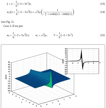
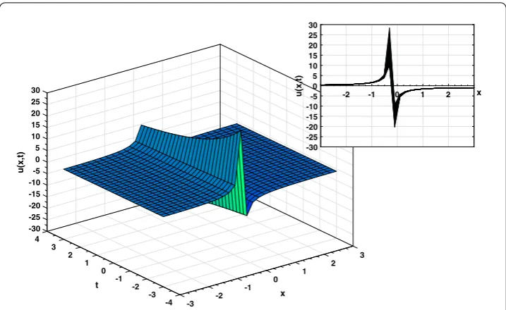
(see Fig. 1). Case2. If we put
a0=
1 6(–2 + 3
√
2λ), a1=
√
2μ, V=1 6
–2 + 3λ2 (15)
Figure 1Exact solutionu1(x,t) of Eq. (2) by substituting the valuesλ= 0.834,μ= 1,α= 0.8, –3≤x≤3,
Figure 2Exact solutionu2(x,t) of Eq. (2) by substituting the valuesλ= 0.834,μ= 1,α= 0.8, –3≤x≤3,
–4≤t≤4,γ= 1 for the 2D graphic
and substitutea0anda1values into (10), we have the following two types of wave solutions
of Eq. (2):
ξ=x+1 6
2 – 3λ2t, (16)
u2(ξ) =
1 6(–2 + 3
√
2λ) +√2μ
1
–μλ+cosh(ξ λ) –sinh(ξ λ)
(17)
(see Fig. 2).
3 Collocation method using radial basis functions
In Eq. (2), ∂∂γtγuis the Caputo fractional derivative throughL1 formula ofu(x,t), which can be written as follows:
∂γu
∂tγ =
⎧ ⎨ ⎩
( t)–γ (2–γ)
n
k=0[unm+1–k–umn–k][(k+ 1)1–γ–k1–γ], n≥1,
( t)–γ
(2–γ)(u1m–u0m), n= 0.
(18)
Now, we discretize the time derivative in (2) by using the Caputo derivative defined in [38] throughL1 formula and the space derivative by the Crank–Nicolson formula between two time levelsnandn+ 1, respectively. Thus, we have
( t)–γ (2 –γ)
n
k=0
unm+1–k–unm–k(k+ 1)1–γ–k1–γ+ 2(uux)
n+1+ (uu
x)n 2
+ 3(u
2u
x)n+1+ (u2ux)n
2 –
un+1
xxx +unxxx
Nonlinear terms of the above equation can be linearized by using the following equations:
By a straightforward computation in Eq. (19), it follows that
2( t)–γ
Now, we shall use radial basis functions.
Radial basis functions are often very variable functions, and their values depend on the distance from the origin. Thusφ(x) =φ(r)∈R,x∈Rnor it is the distance from a point
{xj}ofφ(x–xj) =φ(rj)∈R. We note each function providingφ(x) =φ(x2). In general,
normrj=x–xj2is considered to be the Euclidean distance. Globally supported radial
basis functions throughout the present paper are given as follows:
Multiquadratic (MQ) φ(rj) =
Here,nis the number of data points;φ is some radial basis functions;λjare unknown coefficients defined by collocation methods. Thus, for each collocation point, Eq. (24) be-comes
x, we obtain the following equations:
+ 2 α2are applied. Thus,n×ntype equation systems are obtained in each point of the range
from Eq. (25).
3.1 Stability analysis
In this subsection, we shall investigate the stability of this method with the help of Von-Neumann analysis.
– 6A2αm(n–1,m–1)unm–1+αm(n,m)unm+αm(n+1,m+1)unm+1
+ 3A2αm(n–1,m–1)unm–1+αm(n,m)unm+αm(n+1,m+1)unm+1
+ 3A2αm(n–1+1,m–1)unm–1+αm(n+1,m)unm+αm(n+1+1,m+1)unm+1
–βm(n–1+1,m–1)umn+1–1+βm(n+1,m)umn+1+βm(n+1+1,m+1)unm+1+1
–βm(n–1,m–1)umn–1+βm(n,m)umn +βm(n+1,m+1)unm+1= 0, (29)
whereA=un,B=un x.
Assume the solutions of (29) to be as follows:
un(xm) =ξneϕm, m=m– 1,m,m+ 1, (30)
whereis the imaginary unit andϕis real. Firstly, substituting the Fourier mode (30) into the recurrence relationship (29), we obtain
2( t)–γ (2 –γ)
n
k=0
(k+ 1)1–γ–k1–γξn–k+1–ξn–kei(m–1)ϕ+eimϕ+ei(m+1)ϕ
+2 + 6ABξn+1ei(m–1)ϕ+eimϕ+ei(m+1)ϕ
+2A+ 3A2ξn+1αm(n–1+1,m–1)ei(m–1)ϕ+αm(n+1,m)eimϕ+αm(n+1+1,m+1)ei(m+1)ϕ
– 3ξnA2αm(n–1,m–1)ei(m–1)ϕ+αm(n,m)eimϕ+αm(n+1,m+1)ei(m+1)ϕ
–ξn+1βm(n–1+1,m–1)ei(m–1)ϕ+βm(n+1,m)eimϕ+βm(n+1+1,m+1)ei(m+1)ϕ
–ξnβm(n–1,m–1)ei(m–1)ϕ+βm(n,m)eimϕ+βm(n+1,m+1)ei(m+1)ϕ= 0. (31)
Next, letξn+1=ζ ξnand assume thatζ=ζ(ϕ) is independent of time. Then we easily obtain the following expression:
2( t)–γ (2 –γ)
n
k=0
(k+ 1)1–γ–k1–γξn–k+1–ξn–ke–iϕ+ 1 +eiϕ
–βm(n–1,m–1)e–iϕ+β(n,m)
m +β
(n,m+1)
m+1 eiϕ
– 3A2αm(n–1,m–1)e–iϕ+α(n,m)
m +α
(n,m+1)
m+1 eiϕ
+ξ2A+ 3A2α(mn–1+1,m–1)e–iϕ+α(n+1,m)
m +α
(n+1,m+1)
m+1 eiϕ
–βm(n–1+1,m–1)e–iϕ+β(n+1,m)
m +β
(n+1,m+1)
m+1 eiϕ
+2 + 6ABξn+1e–iϕ+ 1 +eiϕ= 0. (32)
Let us denote Eq. (32) as follows:
|ζ|=X1+iX2 Y1+iY2
where
If|ζ| ≤1 conditional is satisfied, then we see that the proposed method is unconditionally stable.
3.2 L2andL∞error norms
For the test problem used in the present study, numerical solutions of Eq. (2) are computed with help of Mathematica software. BothL2error norms are given by
L2=Uexact–UN2=
They are calculated to show the accuracy of the results.
3.3 Test problem
Forλ= 0.834,μ= 1, –γ = 0.8, the exact solution of the fractional combined KdV–mKdV equation is given as follows:
Table 1 Comparison of the error normsL2andL∞of the obtained solution usingIQradial basis for
h= 0.1andh= 0.01 atc= 10–15, t= 0.01
Numerical solution for
φ(rj) = 1/(r2j+c2)
Exact solution
h= 0.01
x= 0 6.18208 6.64277
x= 0.1 4.14476 4.35567
x= 0.2 3.08694 3.20707
x= 0.3 2.44095 2.51819
x= 0.4 2.00673 2.0604
x= 0.5 1.69576 1.73507
x= 0.6 1.46278 1.49273
x= 0.7 1.28229 1.30578
x= 0.8 1.13878 1.15765
x= 0.9 1.02233 1.03776
x= 1 0.939049 0.939049
L2( t=h= 0.1) 0.0844697
L∞( t=h= 0.1) 3.1226
L2( t=h= 0.01) 0.116856
L∞( t=h= 0.01) 5.90397
Figure 3Comparison of the exact solution and the obtained solutions using IQ, MQ, IMQ bases forh= 0.1
In our computations, the linearization technique has been applied for the numerical solution of the test problem. Then, the numerical tests are performed using the radial basis functionGA,IQ,IMQ,MQ. The collocation matrix does not become ill-conditional during the run algorithms withGAradial basis functions forc= 10–15at Eq. (2). In Table 1,
the error normsL2andL∞of numerical solutions withIQbasis are compared forc= 10–15
and t= 0.01 at timest= 1. In Fig. 3, the numerical solutions obtained byIQ,IMQ,MQ bases are compared forh= 0.1 at timest= 1.
4 Geometry of the exact solution
The geometry of the exact solutions of various equations has been intensely studied by different authors in various ways (cf. [40–44]). In this section, we are going to investigate the exact solution and the numerical solutions in the 3-dimensional space-time known as Lorentz–Minkowski spaceR31. The main reason for choosing to work in this space is that the Lorentz–Minkowski space plays an important role in both special relativity and general relativity with space coordinates and time coordinates.
First, we need to recall some basic facts and notations inR3
1(cf. [45–49]).
LetX= (x1,x2,x3) andY= (y1,y2,y3) be any two vector fields inR31. Then inner product
ofXandY is defined by
X,Y=x1y1+x2y2–x3y3. (35)
Note that a vector fieldXis called
(i) a timelike vector ifX,X< 0, (ii) a spacelike vector ifX,X> 0,
(iii) a lightlike(or degenerate)vector ifX,X= 0andX= 0.
Thus, the inner product in R31 splits each vector field into three categories, namely (i) spacelike, (ii) timelike, and (iii) lightlike (degenerate) vectors. The category is known as causal character of a vector. The set of all lightlike vectors is called null cone. Further-more, the norm of a vectorXis defined by its causal character as follows:
(i) X=√X,XifXis a spacelike vector, (ii) X= –√X,XifXis a timelike vector.
LetXbe a unit timelike vector ande= (0, 0, 1) inR31. ThenXis called
(i) a timelike future pointing vector ifX,e> 0, (ii) a timelike past pointing vector ifX,e< 0.
Now, letr(x,t) be a surface inR13. Then the normal vectorNat a point inr(x,t) is given by
N= rx∧rt rx∧rt
, (36)
where∧denotes the wedge product inR3
1. A surface is called (i) a timelike surface ifNis spacelike,
(ii) a spacelike surface ifNis timelike,
(iii) a lightlike (or degenerate) surface ifNis lightlike.
We note that a point is called regular ifN= 0 and singular ifN= 0. Now, let us consider a surface given by
r(x,t) =x,t,u(x,t), (37)
whereu(x,t) is the exact solution of the fractional combined KdV–mKdV equation given by
u(x,t) =1 6(–2 + 3
√ 2λ)
+√2μ
1
–μλ+cosh((x+16(2 – 3λ2)t)λ) –sinh((x+1
6(2 – 3λ2)t)λ)
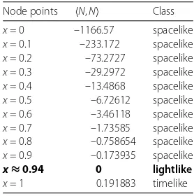
Table 2 Classification ofr(x,t) surface at node points
Node points N,N Class
x= 0 –1166.57 spacelike
x= 0.1 –233.172 spacelike
x= 0.2 –73.2727 spacelike
x= 0.3 –29.2972 spacelike
x= 0.4 –13.4868 spacelike
x= 0.5 –6.72612 spacelike
x= 0.6 –3.46118 spacelike
x= 0.7 –1.73585 spacelike
x= 0.8 –0.758654 spacelike
x= 0.9 –0.173935 spacelike
x≈0.94 0 lightlike
x= 1 0.191883 timelike
In view of (36), the normal vector field ofr(x,t) becomes
N(x,t) = (e2λ3t–λ3t+2λx18eλ3t–23λ(t+3x)λ4– 72eλ3t–λ 3t 2 t+λxλμ3
+ 18e23λt–λ3t+2λxμ4–λ2μ72e16λ((–2+3λ2)t–6x)λ
+–108 + 40λ4– 12λ6+ 9λ8μ/18λ–eλ(16(2–3λ2)t+x)μ4. (38)
From (38), it is clear thatr(x,t) is a regular surface, that is, every point of it is a regular point.
As a consequence of the above facts, we immediately get the following.
Corollary 4.1 For the node points,we have Table2.
Remark4.2 From Table 2, we see that the surfacer(x,t) contains at least one degenerate point nearx= 0.94. As the number of node points increases, we approach degenerate points. Therefore, numerical solutions become instable when the number of node points increases.
5 Gaussian curvature of node points
Another important fact for a surface is to compute the Gaussian curvature which is an intrinsic character of it. The Gaussian curvature is the determinant of the shape opera-tor. For a surfacer(x,t), we shall apply the following useful way to compute the Gaussian curvature:
ConsiderN,N=εN, whereε=∓1. Let us define
E=rx,rx, F=rx,rt, G=rt,rt (39)
and
e=uxx,N, f =uxt,N, g=utt,N.
Then the Gaussian curvatureK(p) at a pointpof a surface satisfies
K(p) =ε eg–f 2
We note that
(i) K(p) > 0means that the surfacer(x,t)is shaped like an elliptic paraboloid nearp. In this case,pis called an elliptic point.
(ii) K(p) < 0means that the surfacer(x,t)is shaped like a hyperbolic paraboloid nearp. In this case,pis called a hyperbolic point.
(iii) K(p) = 0means that the surfacer(x,t)is shaped like a parabolic cylinder or a plane nearp. In this case,pis called a parabolic point.
Now, let us consider the surface given in (37). From (39) and (40), by a straightforward computation, we get
K= –e4λ3t+λ3t+4λxλ82 – 3λ22–8 + 3λ24 + 3λ2μ2eλ3tλ2
–e23λ(t+3x)μ22/2eλ(t+λ2t+3x)λ2–108 + 40λ4– 12λ6+ 9λ8μ2
– 18eλ3t+λxμ4+ 18eλ 3t 2 λe3λ
3t
2 λ3– 4eλ((13+λ2)t+x)λ2μ– 4eλ(t+3x)μ3
eλ(t+λ2t+3x)λ2108 + 40λ4– 12λ6+ 9λ8μ2
+ 18eλ3t+λxe2λ3tλ4– 4e16λ(2+9λ2)t+λxλ3μ– 4eλt+λ 3t
3 +3λxλμ3+e43λ(t+3x)μ4.
Another important kind of curvatures is mean curvature which measures the surface tension from the surrounding space at a point. The mean curvature is a trace of the second fundamental form. For a surfacer(x,t), we shall apply the following useful way to compute the mean curvatureH(p):
H(p) =ε1
2
eG– 2fF+gE
EG–F2 . (41)
IfH(p) = 0 for all points ofr(x,t), then the surface is called minimal. Furthermore, if the value of the mean curvature at a pointpreceives at least a possible amount of tension from the surrounding space, thenpis called ideal point. That is, if a point in a surface is affected as little as possible from the external influence, then it becomes ideal.
From (41), we obtain
H=3eλ3t–λ 3t
2 +λxλ440 – 12λ2+ 9λ4
μλ+eλ(16(2–3λ2)t+x)μ/2λ–eλ(16(2–3λ2)t+x)μ3
1/λ–eλ(16(2–3λ2)t+x)μ4e2λ3t–λ3t+2λx
–18eλ3t–2λ(t3+3x)λ4+ 72eλ3t–λ 3t 2 +λxλμ3
– 18e2λ3t–λ3t+2λxμ4+λ2μ72e16λ((–2+3λ2)t–6x)λ
+–108 + 40λ4– 12λ6+ 9λ8μ3/2).
As a consequence of the above facts, we get the following corollary:
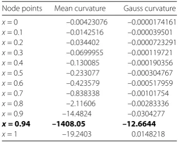
Corollary 5.1 For the node points of r(x,t),we have Table3.
Table 3 Curvatures ofr(x,t) surface at node points
Node points Mean curvature Gauss curvature
x= 0 –0.00423076 –0.0000174161
x= 0.1 –0.0142516 –0.000039501
x= 0.2 –0.034402 –0.0000723291
x= 0.3 –0.0699955 –0.000119721
x= 0.4 –0.130085 –0.000190356
x= 0.5 –0.233077 –0.000304767
x= 0.6 –0.423579 –0.000517959
x= 0.7 –0.838338 –0.00101754
x= 0.8 –2.11606 –0.00283336
x= 0.9 –14.4824 –0.0304277
x = 0.94 –1408.05 –12.6644
x= 1 –19.2403 0.0148218
6 Conclusions
Using the (1/G) expansion method, the exact solutionr(x,t) of the fractional combined KdV–mKdV equation is obtained. The numerical solutions of the fractional combined KdV–mKdV equation are shown by using the collocation method. These solutions are compared with the exact solution. The computational efficiency and effectiveness of the proposed method were tested on a problem. The error normsL2andL∞ have been
cal-culated. The obtained results show that the error norms are small during all computer runs for all bases except for MQ basis. It was proved that the present method is a particu-larly successful numerical scheme to solve the fractional combined KdV–mKdV equation. However, numerical solutions are more accurate forh= 0.1 than forh= 0.01. Therefore, casual character of the exact solution was expressed at the nodal points. From Tables 1 and 2, it was realized that the most accurate numerical solution occurred in the timelike case ofr(x,t), and there exists at least one degenerate point nearx= 0.94. Furthermore, from Table 3, it was realized that the most accurate numerical solution occurred at the elliptic points ofr(x,t), and the ideal node point ofr(x,t) isx= 0.
Acknowledgements
The authors are thankful to the referees for their valuable comments and constructive suggestions towards the improvement of the paper.
Competing interests
The authors declare that they have no competing interests.
Authors’ contributions
All authors contributed equally to the writing of this paper. All authors read and approved the final manuscript.
Author details
1Department of Mathematics, Faculty of Science and Art, Istanbul Ticaret University, Istanbul, Turkey.2Department of
Actuary, Faculty of Science and Art, Firat University, Elazı ˘g, Turkey.3Department of Mathematics, Faculty of Science and
Art, Siirt University, Siirt, Turkey.
Publisher’s Note
Springer Nature remains neutral with regard to jurisdictional claims in published maps and institutional affiliations.
Received: 14 November 2017 Accepted: 15 February 2018
References
1. Das, S.: Functional Fractional Calculus. Springer, Berlin (2011)
2. Agarwal, R.P., Benchohra, M., Hamani, S., Pinelas, S.: Boundary value problems for differential equations involving Riemann–Liouville fractional derivative on the half line. Dyn. Contin. Discrete Impuls. Syst., Ser. A Math. Anal.18(2), 235–244 (2011)
4. Kaya, D., Yoku¸s, A.: Stability analysis and numerical solutions for time fractional KdVb equation. In: International Conference on Computational Experimental Science and Engineering, Antalya (2014)
5. Khater, A., Helal, M., El-Kalaawy, O.: Bäcklund transformations: exact solutions for the KdV and the Calogero–Degasperis–Fokas mKdV equations. Math. Methods Appl. Sci.21(8), 719–731 (1998)
6. Kumar, D., Singh, J., Baleanu, D., et al.: Analysis of regularized long-wave equation associated with a new fractional operator with Mittag–Leffler type kernel. Phys. A, Stat. Mech. Appl.492, 155–167 (2018)
7. Kumar, D., Singh, J., Baleanu, D.: A new fractional model for convective straight fins with temperature-dependent thermal conductivity. Therm. Sci.1, 1–12 (2017)
8. Momani, S., Noor, M.A.: Numerical methods for fourth-order fractional integro-differential equations. Appl. Math. Comput.182(1), 754–760 (2006)
9. Momani, S., Odibat, Z.: Homotopy perturbation method for nonlinear partial differential equations of fractional order. Phys. Lett. A365(5), 345–350 (2007)
10. Safari, M., Ganji, D., Moslemi, M.: Application of He’s variational iteration method and Adomian’s decomposition method to the fractional KdV–Burgers–Kuramoto equation. Comput. Math. Appl.58(11), 2091–2097 (2009) 11. Sakar, M.G., Akgül, A., Baleanu, D.: On solutions of fractional Riccati differential equations. Adv. Differ. Equ.2017(1), 39
(2017)
12. Singh, J., Kumar, D., Baleanu, D.: On the analysis of chemical kinetics system pertaining to a fractional derivative with Mittag–Leffler type kernel. Chaos, Interdiscip. J. Nonlinear Sci.27(10), 103113 (2017)
13. Song, L., Zhang, H.: Application of homotopy analysis method to fractional KdV–Burgers–Kuramoto equation. Phys. Lett. A367(1), 88–94 (2007)
14. Wei, L., He, Y., Yildirim, A., Kumar, S.: Numerical algorithm based on an implicit fully discrete local discontinuous Galerkin method for the time-fractional KdV–Burgers–Kuramoto equation. Z. Angew. Math. Mech.93(1), 14–28 (2013)
15. Choi, J., Kumar, D., Singh, J., Swroop, R.: Analytical techniques for system of time fractional nonlinear differential equations. J. Korean Math. Soc.54(4), 1209–1229 (2017)
16. Kumar, D., Singh, J., Baleanu, D.: A new numerical algorithm for fractional Fitzhugh–Nagumo equation arising in transmission of nerve impulses. Nonlinear Dyn.91, 307–317 (2018)
17. Baleanu, D., Jajarmi, A., Hajipour, M.: A new formulation of the fractional optimal control problems involving Mittag–Leffler nonsingular kernel. J. Optim. Theory Appl.175(3), 718–737 (2017)
18. Baleanu, D., Jajarmi, A., Asad, J., Blaszczyk, T.: The motion of a bead sliding on a wire in fractional sense. Acta Phys. Pol. A131(6), 1561–1564 (2017)
19. Hajipour, M., Jajarmi, A., Baleanu, D.: An efficient nonstandard finite difference scheme for a class of fractional chaotic systems. J. Comput. Nonlinear Dyn.13(2), 021013 (2018)
20. Jajarmi, A., Hajipour, M., Baleanu, D.: New aspects of the adaptive synchronization and hyperchaos suppression of a financial model. Chaos Solitons Fractals99, 285–296 (2017)
21. Miller, K.S., Ross, B.: An Introduction to the Fractional Calculus and Fractional Differential Equations (1993) 22. Aslan, E.C., Inc, M., Qurashi, M.A., Baleanu, D.: On numerical solutions of time-fraction generalized Hirota Satsuma
coupled KdV equation. J. Nonlinear Sci. Appl.10(2), 724–733 (2017)
23. Bandyopadhyay, S.: A new class of solutions of combined KdV–mKdV equation. arXiv preprint (2014). arXiv:1411.7077 24. Djoudi, W., Zerarka, A.: Exact solutions for the KdV–mKdV equation with time-dependent coefficients using the
modified functional variable method. Cogent Math.3(1), 1218405 (2016)
25. Jafari, H., Tajadodi, H., Baleanu, D., Al-Zahrani, A.A., Alhamed, Y.A., Zahid, A.H.: Exact solutions of Boussinesq and KdV–mKdV equations by fractional sub-equation method. Rom. Rep. Phys.65(4), 1119–1124 (2013)
26. Kaya, D., Inan, I.E.: A numerical application of the decomposition method for the combined KdV–mKdV equation. Appl. Math. Comput.168(2), 915–926 (2005)
27. Krishnan, E., Peng, Y.-Z.: Exact solutions to the combined KdV–mKdV equation by the extended mapping method. Phys. Scr.73(4), 405–409 (2006)
28. Lu, D., Shi, Q.: New solitary wave solutions for the combined KdV–mKdV equation. J. Inf. Comput. Sci.8(7), 1733–1737 (2010)
29. Sierra, C.G., Molati, M., Ramollo, M.P.: Exact solutions of a generalized KdV–mKdV equation. Int. J. Nonlinear Sci.13(1), 94–98 (2012)
30. Triki, H., Taha, T.R., Wazwaz, A.-M.: Solitary wave solutions for a generalized KdV–mKdV equation with variable coefficients. Math. Comput. Simul.80(9), 1867–1873 (2010)
31. Golbabai, A., Nikan, O.: A meshless method for numerical solution of fractional differential equations. Casp. J. Math. Sci.4(1), 1–8 (2015)
32. Rong-Jun, C., Yu-Min, C.: A meshless method for the compound KdV–Burgers equation. Chin. Phys. B20(7), 070206 (2011)
33. Hu, H.-Y., Li, Z.-C., Cheng, A.H.-D.: Radial basis collocation methods for elliptic boundary value problems. Comput. Math. Appl.50(1–2), 289–320 (2005)
34. Hon, Y., Schaback, R.: On unsymmetric collocation by radial basis functions. Appl. Math. Comput.119(2), 177–186 (2001)
35. Haq, S., Uddin, M., et al.: Numerical solution of nonlinear Schrodinger equations by collocation method using radial basis functions. Comput. Model. Eng. Sci.44(2), 115–136 (2009)
36. Šarler, B., Vertnik, R., Kosec, G., et al.: Radial basis function collocation method for the numerical solution of the two-dimensional transient nonlinear coupled Burgers equations. Appl. Math. Model.36(3), 1148–1160 (2012) 37. Yokus, A., Kaya, D.: Numerical and exact solutions for time fractional Burgers’ equation. J. Nonlinear Sci. Appl.10(7),
3419–3428 (2017)
38. Oldham, K., Spanier, J.: The Fractional Calculus. Academic Press, New York (1974)
39. Golbabai, A., Mohebianfar, E.: A new stable local radial basis function approach for option pricing. Comput. Econ.
49(2), 271–288 (2017)
40. Sasaki, R.: Soliton equations and pseudospherical surfaces. Nucl. Phys. B154(2), 343–357 (1979)
42. Altalla, F.H.: Exact solution for some nonlinear partial differential equation which describes pseudo-spherical surfaces. PhD thesis, Zarqa University (2015)
43. Matveev, V.B., Matveev, V.: Darboux Transformations and Solitons (1991)
44. Rogers, C., Schief, W.K.: Bäcklund and Darboux Transformations: Geometry and Modern Applications in Soliton Theory. Cambridge Texts in Applied Mathematics, vol. 30. Cambridge University Press, Cambridge (2002) 45. Duggal, K.L., Bejancu, A.: Lightlike Submanifolds of Semi-Riemannian Manifolds and Applications. Mathematics and
Its Applications, vol. 364. Springer, Dordrecht (2013)
46. Duggal, K.L., Jin, D.H.: Null Curves and Hypersurfaces of Semi-Riemannian Manifolds. World Scientific, Singapore (2007)
47. Duggal, K.L., Sahin, B.: Differential Geometry of Lightlike Submanifolds. Springer, Basel (2011)
48. López, R.: Differential geometry of curves and surfaces in Lorentz–Minkowski space. arXiv preprint (2008). arXiv:0810.3351