R E S E A R C H
Open Access
Quantized Network Coding for correlated
sources
Mahdy Nabaee
*and Fabrice Labeau
Abstract
In this paper, we present a data gathering technique for sensor networks that exploits correlation between sensor data at different locations in the network. Contrary to distributed source coding, our method does not rely on knowledge of the source correlation model in each node although this knowledge is required at the decoder node. Similar to network coding, our proposed method (which we call Quantized Network Coding) propagates mixtures of packets through the network. The main conceptual difference between our technique and other existing methods is that Quantized Network Coding operates on the field of real numbers and not on a finite field. By exploiting principles borrowed from compressed sensing, we show that the proposed technique can achieve a good approximation of the network data at the sink node with only a few packets received and that this approximation gets progressively better as the number of received packets increases. We explain in the paper the theoretical foundation for the algorithm based on an analysis of the restricted isometry property of the corresponding measurement matrices. Extensive simulations comparing the proposed Quantized Network Coding to classic network coding and packet forwarding scenarios demonstrate its delay/distortion advantage.
Keywords: Linear network coding; Distributed source coding; Compressed sensing; Restricted isometry property;
1minimization
1 Introduction
Flexible, low cost, and long-lasting implementation of wireless sensor networks has made them an unavoidable alternative for conventional wired sensing structures in a wide variety of applications, including medicine, trans-portation, and military [1]. As a relatively new technology, more challenges are faced in the networking aspects of communication than in the aspects of classic physical [2]. One of the introduced challenges is the gathering of sensed data at a central node of the network, where deliv-ery delay, precision, and robustness to network changes are emerging issues.
Packet forwarding via routing is widely used in differ-ent implemdiffer-entations of sensor networks. While it achieves capacity rates in the case of multiple session unicast in lossless networks [3], packet forwarding requires an appropriate routing [4] protocol to be run. However, packet forwarding can lead to difficulties because of
*Correspondence: [email protected]
Department of Electrical and Computer Engineering, McGill University, Montreal, QC, Canada
its slow adaptation to the network changes, caused by deploying new node(s) or link failure(s).
Further, in the case of lossy networks, network coding offers a better error correction capability than packet for-warding, as a result of network diversity. Network coding [3] has been proposed as an alternative for packet for-warding in sensor networks [5,6]. Specifically, network coding sends a function of incoming packets to the inter-mediate nodes, as opposed to sending their original con-tent. Furthermore, the usage of random linear functions, also known as random linear network coding, is proved to be sufficient in lossless networks [7,8]. Moreover, the-oretical analysis shows that when network coding is used for transmission, no queuing is required to achieve the capacity rates of the network [3]. Network coding in lossy networks can result in improved achieved rate regions, compared to packet forwarding [9,10].
In the case of correlated sources, distributed source cod-ing [11,12] on top of packet forwardcod-ing is proved to be sufficient, when dealing with networks of lossless links [13]. Similar to packet forwarding, network coding can be separately applied on top of distributed source coding
for correlated sources [14,15]. However, one has to per-form joint source network decoding in order to achieve theoretical performance limits, which may not be feasi-ble because of its computational complexity [15]. Different solutions have been proposed to tackle this practicality issue [16-18], by using low-density codes and sum product algorithm [19] for decoding.
Distributed source coding requires the availability of appropriate marginal coding rates at each encoder node; similarly, the deployment of joint source network decod-ing requires some knowledge of the correlation model of the sources on the encoding side. The assumption of this knowledge might not be practical in all cases, even more so when the source characteristics change over time.
Motivated by this observation, we aim to develop a data gathering and transmission scheme that, similar to net-work coding, does not rely on routing but at the same time can intrinsically take advantage of the source corre-lation. Our approach models source correlation through a sparsity or compressibility assumption; combined with a specific data gathering scheme inspired by network cod-ing but actcod-ing in the real field, this assumption allows us to develop recovery algorithms at the sink node, which allow approximate data recovery with low delay. Our recov-ery mechanism will be based on ideas borrowed from compressed sensing [20,21] in which the inter-node corre-lation model of the messages, interpreted as near-sparsity in some domain, is used.
Recently, the idea of using compressed sensing and sparse recovery concepts in sensor networks has drawn a lot of attention [22-25]. Specifically, with the aid of the compressed sensing concepts, compression of inter-node correlated data without using their correlation model is done in [22,23]. Morevoer, in [26,27], theoretical discus-sion on sparse recovery of graph constrained measure-ments with an interest in network monitoring application is presented. Joint source, channel, and network coding was also proposed in [28], where random linear mixing was proposed for compression of temporally and spatially correlated sources. In [29], practical possibility of finite field network coding of highly correlated sources was investigated, with the aid of low-density codes and belief propagation-based decoding. Unfortunately, a solid theo-retical investigation on the feasibility of adopting sparse recovery in random linear network coding has not been done previously.
Real network coding has shown interesting advan-tages over the conventional finite field network coding [30]. In our earlier work [31], we combined the idea of using real field network coding with the concepts of compressed sensing and proposed a non-adaptive
dis-tributed compression scheme, calledQuantized Network
Coding (QNC), for exactly sparse sources. Furthermore, in [32], we initiated a discussion on the theoretical
feasibility of compressed sensing-based network coding, using restricted isometry property of random matrices. In this paper, we extend our previous work from [31,32] in two specific ways: (i) we extend the network source model used from exactly sparse to near-sparse signals, and (ii) we provide a detailed mathematical and numer-ical justification of the usage of sparse recovery algo-rithms (including a bound on the reconstruction error) for this source model. Finally, extensive computer sim-ulations are used to compare the performance of the proposed QNC scenario with respect to other network transmission scenarios. Specifically, our focus is to study the distributed compression capabilities of the proposed QNC scenario in a lossless scenario. The study of robust transmission in lossy cases will be done in a future work.
Although the idea of using compressed sensing has been initially proposed in [22], its theoretical and practical possibilities have not been studied by providing a math-ematical formulation. Additionally, we discuss on using compressed sensing in a network coding-based scenario, which involves quantization and is different from the work in [22].
As another contribution of our work, we discuss the sat-isfaction of RIP in a network coding scenario, which has not been addressed in other works. Specifically, in [25,28], the authors do not discuss explicit conditions for which compressed sensing encoding (and decoding) works prop-erlya. In this work, we propose conditions for network coding coefficients which ensure a robust recovery of messages, by using restricted isometry property.
2 Problem description and notation
In this paper, we limit our study to a network with loss-less links with limited capacity. This model could also correspond to lossy networks, where appropriate channel coding would have been applied. A more realistic lossy network model is left as a future work.
2.1 Network
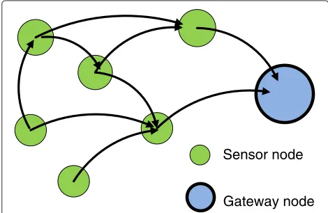
As shown in Figure 1, we represent the network by a directed graph,G = (V,E), whereV andE are the sets of nodes (vertices) and directed edges (links). Each node,
v, is from the finite sorted setV = {1,. . .,n}, and each edge,e, is from the finite sorted setE = {1,. . .,|E|}. Fur-ther, each edge (link) can maintain a lossless transmission from tail(e)to head(e), at a maximum finite rate ofCebits
per use. Transmission over each link is assumed to have no interference involved from other links or nodes. One may modify the capacities of each link to reflect the effect of interference over each link.
We define the sets of incoming and outgoing edges of nodev, denoted by In(v) and Out(v), respectively, as follows:
In(v)= {e:e∈E, head(e)=v}, (1)
Out(v)= {e:e∈E, tail(e)=v}. (2)
The content of edgeeat time instanttare represented by
Ye(t), wheretrepresents the discrete (integer) time index,
during which a block ofLchannel symbolsbis transmit-ted.Ye(t)is from a finite alphabet of size2LCe, where
denotes rounding down to the nearest integer. In the rest of the paper, the realizations of all capital letter random variables are denoted by lowercase letters.
2.2 Source signals
The nodes of the network are equipped with sensors; specifically, we model the sensed signals in each nodevas
Sensor node
Gateway node
Figure 1Directed graph representing a data gathering sensor network.
an information source,Xv, whereXv ∈ R. To reflect the
natural correlation between sensed data at each node, we assume that the set of signalsXvare near-sparse in some
transform domain.
More specifically, defining the sorted vectorcofXv’s,
X=[Xv:v∈V] , (3)
we assume that X is near-sparse in some orthonormal
transform domainφn×n. Explicitly, forS = φT·X, and a
small positivek, we have S−Sk
1 S
1
≤k, (4)
whereSkis such that Sk
0 =k, (5)
i.e.,Sk isk-sparse. An example of the sparsifying trans-form matrix,φ, is the Karhunen Loeve transform of the messages.
Moreover, we assume that messages,Xv’s, take their
val-ues in a bounded interval between−qmaxand+qmax. This is also a reasonable assumption as the sensing range of sensors is usually limited. The choice ofqmaxcan be made after a statistical study of realizations ofXv’s and can be
chosen as some confidence region, in which most of the realizations ofXv’s lay. Note that the sparsity model used
in this paper is different from the conventional joint sparse model (JSM) [35], in that our node source signals or mes-sagesare scalar random variables, without correlation over time in each node. This is a valid assumption as a local transform coding could be applied to the time samples and generate a set of samples with no time redundancy.
2.3 Data gathering
Having these correlated information sources and the information network characterized, we study the trans-mission ofXv’s to a single gateway node. The gateway or
decoder node, denoted byv0,v0 ∈ V, has high compu-tational resources and is usually in charge of forwarding the information to a next level network, e.g., a wired back-bone network. The described (single session) incast of sources to the unique decoder node is referred to asdata gathering.
3 Quantized Network Coding 3.1 Principle
On the other hand, the finite capacity of the edges has to be appropriately coped with. As a result, we propose a method that we callQuantized Network Coding, which uses quantization to match infinite alphabet of real field network coded packets to the limited capacity of the network links.
In [31], for each network nodev∈Vand each outgoing edgee∈Out(v), we defined QNC at nodev, according to
condition in the network. This means that, at timet, the message on any outgoing edge of a node is made up of a quantized linear combination of the messages received by the node at the previous time instant and the information
Xvmeasured by the node. The messages,Xv’s, are assumed
to be constant until the transmission is complete, which is whyXv’s do not depend ont. The local network coding
coefficients,βe,e(t)’s andαe,v(t)’s, are real-valued, and the
determination of their value will be discussed in Section 4. The quantizer operator,Qe(), corresponding to outgoing edgee, is designed based on the values ofCeandL, and the
distribution of its input (i.e., random linear combinations). A simple diagram of QNC at nodevis shown in Figure 2.
3.2 End-to-end equations
Figure 2A simple diagram of Quantized Network Coding.
{A(t)}e,v=
αe,v(t), tail(e)=v
0, otherwise . (9)
We also define the vectors of edge contents,Y(t), and quantization noises,N(t), according to
Y(t)=[Ye(t):e∈E] , (10) N(t)=[Ne(t):e∈E] . (11)
As a result, (7) can be re-written in the following form:
Y(t)=F(t)·Y(t−1)+A(t)·X+N(t). (12)
Depending on the network deployment, matrix
[B]|In(v0)|×|E|defines the relation between the content of edges,Y(t), and the received packets at the decoder node
v0. Explicitly, we define the vector of received packets at
timetat the decoder:
Z(t)=[Ye(t):e∈In(v0)]=B·Y(t), (13)
By considering (12) as the difference equation, charac-terizing a linear system withXandN(t)’s as its inputs, and
Z(t)its output, and using the results in [36], one gets
Z(t)=(t)·X+Neff(t), (15)
where the measurement matrix, (t), and the effective noisevector,Neff(t), are calculated as follows:
(t)=B·
andIdenotes the identity matrix.
where them×n total measurement matrix,tot(t), and
the total effective noise vector, Neff,tot(t), are the con-catenation result of measurement matrices, (t)’s, and effective noise vectors,Neff(t). Because of our assumption to start transmission fromt = 1, measurements inZ(1) are not useful for decoding, and therefore
tot(t)=
In conventional linear network coding, the total num-ber of measurements,m(see (19)), is at least equal to the
number of data sources,n(the number of nodes in the
network here). Typically, the total measurement matrix is of full column rank, and if there is no uncertainty involved because of measurement noise, we are able to uniquely find a solution. In this paper, we are interested in investi-gating the feasibility of robust recovery ofX, when fewer number of measurements are received at the decoder than the number of messages, i.e.,m<n.
The characteristic Equation (20) describing the QNC scenario can be treated as a compressed sensing measure-ment equation. This gives us an opportunity to apply the results in the literature of compressed sensing and sparse recovery [20,37] to our QNC scenario with near-sparse messages. However, one needs to examine the required conditions which guarantee sparse recovery in the pro-posed QNC scenario. In the following, we discuss theo-retical and practical feasibility of robust recovery with a compressed sensing perspective.
4 Restricted isometry property
One of the main advantages of the compressed sensing approach is that it relies on a simple model of correlation for the sources; if sparse reconstruction can be applied successfully to recoverXfrom Equation 20 at a given time
t, this is achieved without requiring the encoders (net-work nodes) to know much about the underlying signal correlation. This section discusses the design of the lin-ear mixing coefficientsαe,v(t)andβe,e(t)and the impact
of this design on the ability to apply sparse reconstruction techniques at the sink nodev0 to approximately recover
then source signalsX from mmeasurements Z(t) at a given timet, wherem n.
4.1 The restricted isometry property
One of the properties that is widely used to character-ize appropriate measurement matrices in the compressed
sensing literature is therestricted isometry property(RIP) [33]. Roughly speaking, this property provides a measure of norm conservation under dimensionality reduction [34]. In compressed sensing, the RIP of the measurement matrix between the sparse domain and the measure-ment domain allows to draw strong conclusions about the possibility to recover the original data from a small set of measurements [33]. In our case, this means that the RIP should hold for the measurement matrix tot(t) =
tot(t)φ.
Random matrices with i.i.d. zero-mean Gaussian entries are known to be appropriate measurement matrices for compressed sensing. Explicitly, anm× n i.i.d Gaussian random matrix, denoted G, with entries of variance m1, satisfies RIP of orderkand constantδk, with a probability
exceeding 1−e−κ1m, (calledoverwhelmingprobability) if m> κ2klog(nk), whereκ1andκ2only depend on the value
ofδk(theorem 5.2 in [38]).
Using the results above, it can be understood that an
m×ni.i.d Gaussian random matrix,G, satisfies RIP of orderk, with a high probability, when the order of number of measurements,m, isklog(n/k), formally writing:
which is smaller than the order of n, the size of the data [38].
4.2 QNC design for RIP
We now turn to the design of QNC coefficients in Equation 6 so that the overall design satisfies RIP with high probability. We assemble here several results from the literature and additional simulations to motivate the proposed design.
In [31,32], we proposed a design for local network cod-ing coefficients, βe,e(t)’s and αe,v(t)’s, which results in
an appropriate total measurement matrix,tot(t), in the
compressed sensing framework.
Theorem 1(Theorem 3.1 in [32]).Consider a Quan-tized Network Coding scenario, in which the network cod-ing coefficients,αe,v(t)andβe,e(t), are such that:
• αe,v(t)=0, ∀t>2.
• αe,v(2)’s are independent zero-mean Gaussian random variables.
For such a scenario, the entries of the resultingtot(t) are zero-mean Gaussian random variables. Further, the entries of different columns of tot(t)are mutually inde-pendent.
It is also numerically shown in [32] that a locally orthog-onal set ofβe,e(t)’s is a better choice than non-orthogonal
setsd. This choice of coefficients is defined, for each node
vand for alle,e∈Out(v), as
In cases where the number of outgoing edges is greater than the number of incoming edges, i.e., |Out(v)| > |In(v)|, some of the outgoing edges are randomly removed (not used for transmission) to ensure that the generated βe,e(t)’s are locally orthogonal. Furthermore, the second
equation in (25) is a coefficient normalization which has no specific impact at this stage of the analysis, but which will be important in the study of bounds on sparse recov-ery performance in Section 5. Heuristically, such choice of orthogonal set makes each outgoing packets (of each node) to be innovative.
In [32], we established the relation between the satisfac-tion of RIP and the so-called tail probability
ptail(tot(t),ε)=max
by proving the following theorem.
Theorem 2(Theorem 4.1 in [32]).Considertot(t)with the tail probability, as defined in (26), and an orthonormal transform matrix φ. Then, tot(t) = tot(t) · φ satis-fies RIP of order k and constant δk, with a probability exceeding,
In [32], we have derived a detailed expression of the tail probability (26). Our ultimate goal would be to use this expression to directly conclude that the number of
necessary measurements m in the QNC scenario is of
the same order as that of a well-known Gaussian mea-surement matrix, as defined above. However, the rela-tionship between the network and QNC parameters on
the one hand and the measurement matrix tot(t) on
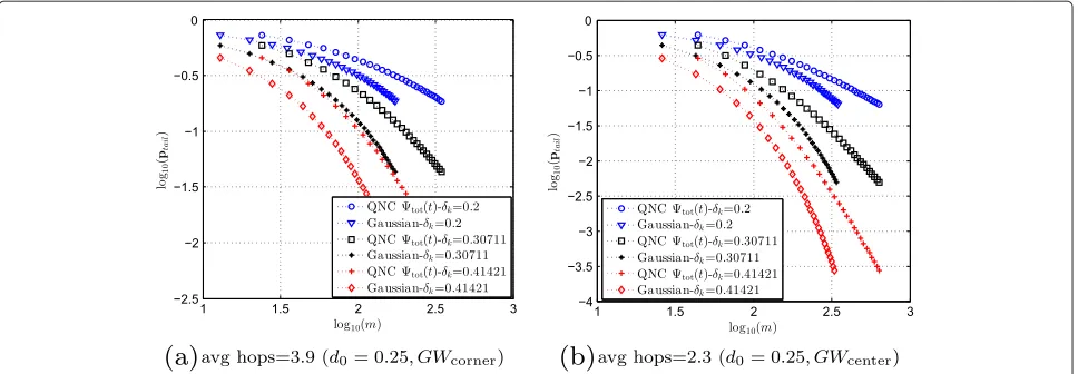
the other hand is too complicated to easily draw conclu-sions (see Equations 8, 9, and 16). We therefore resort to the following reasoning: we first show through sim-ulations that the tail probabilities for the QNC and Gaussian measurement matrices are of the same order; we then conclude to a similar behavior of QNC and Gaussian measurement matrices in terms of RIP satis-faction and thus in terms of the required number of measurements.
In Figure 3, we present the numerical values of tail probabilities (defined in (26)) for the QNC measurement matrix tot(t), ptail(tot(t),ε), using the local network
coding coefficients proposed in Theorem 1 withβe,e(t)’s
satisfying the locally orthogonal conditioneof (25). These tail probabilities are compared with those of i.i.d. Gaus-sian matrices,G, versus the number of measurements,m, in each case.
Our numerical evaluations in Figure 3 show that for the same value of tail probability, the QNC measurement matrix,tot(t), and the i.i.d. Gaussian matrix,G, require a
number of measurementsmof the same order.
We can therefore also say, using Theorem 2, that the QNC measurement matrix,tot(t), and the i.i.d. Gaussian
matrix, G, have a similar behavior in terms of satisfying RIP as a function ofm, so that they will typically require values ofmof the same order to ensure sparse recovery.
In the following section, we extend our discussion to the robust recovery in QNC scenario, by using the guarantees, implied from the satisfaction of RIP.
5 Decoding using sparse recovery
In this section, we will explore the performance of decod-ing usdecod-ing sparse recovery based on Equation 20 and the QNC design proposed in Theorem 1. It is well known that recovery of exactly sparse vectors from an under-determined set of linear measurements can be done with no error, using linear programming [39]. Specifically,
the-oretical works show that the NP-hard 0 minimization
can be replaced with1minimization without any
asso-ciated error, when dealing with noiseless measurements [37,39]. However, when dealing with noisy measurements, 1-min recovery does not necessarily offer a minimum
Figure 3Numerical values of tail probabilities.Logarithmic tail probability versus logarithmic ratio of minimum required number of measurements in our QNC scenario and i.i.d. Gaussian measurement matrices, forn=100 nodes, different RIP constants, and different degrees of nodes. The explanation of network deployments for which tail probabilities are calculated is presented in Section 6.(a)Average hops=3.9 (d0=0.25, GWcorner).(b)Average hops=2.3 (d0=0.25, GWcenter).
Along the lines of [20,33], the compressed sensing-based decoder for the QNC scenario solves the following convex optimization:
ˆ
X(t)=φ·arg min
S S
1,
subject toZtot(t)−tot(t) φS2 ≤rec(t)
(28)
which can be solved by using linear programming [39]. The following theorems present our results on the recov-ery error using1-min decoding of (28).
Theorem 3.Consider the QNC scenario where the abso-lute value of messages are bounded by qmaxand the local network coding coefficients are such that:
• αe,v(t)=0, ∀t>2.
• αe,v(2)’s are independent zero-mean Gaussian random variables with varianceσ02.
• βe,e(t)’s are deterministic and locally orthogonal according to (25).
In such scenario, overflowing of linear combinations (over the limit of qmax) within the nodes happens with a proba-bility less than or equal to
2|E|Q(σ0−1), (29)
where Q()is the tail probability of standard normal dis-tributions (i.e., one-sided Q function).
Proof.Using Cauchy-Schwartz inequality, fort ≥3, we have
e∈In(v)
|βe,e(t)| ≤ ⎛
⎝
e∈In(v)
|βe,e(t)|2 ⎞ ⎠
⎛
⎝
e∈In(v)
1 ⎞ ⎠ 2
(30)
=
1
|In(v)|2
(|In(v)|)2=1 (31)
As a result, sinceαe,v(t)’s are zero fort≥3, it is
straight-forward to imply that overflow may not happen fort ≥
3.
Fort=2, since only the node messageXvis available at
each node, the values ofβe,e(2)’s do not affect anything.
Hence, only the value of αe,v(2) can result in overflow
and therefore|αe,v(2)|should be less than or equal to one
to prevent overflow. Moreover, because of the Gaussian distribution of αe,v(2)’s, each αe,v(2) may have an
abso-lute value more than one, with a probability of 2Q(σ0−1). Therefore, using the union bound, the probability that there is at least oneαe,v(2) with|αe,v(2)| > 1 is upper
bounded by 2|E|Q(σ0−1).
Theorem 4.Consider a QNC scenario where, for all v ∈ V, the network coding coefficients satisfy the condi-tions in Theorem 3, and for which, based on the discussion in Section 4, the measurement matrixtot(t) = tot(t)φ satisfies RIP of order2k with constantδ2k <
√
2−1. The edge quantizers,Qe()’s, are assumed to be uniformf with the step sizee. Then, with a probability exceeding
for the1-min decoding of (28), we have The constants c1and c2are also defined as follows:
c1=4
Proof. According to Theorem 3, the conditions on the local network coding coefficients ensures that
over-flow does not happen with a probability exceeding 1 −
2|E|Q(σ0−1). Further, since the network is lossless, the only associated measurement noise is resulting from the quan-tization noise at the edges. For each uniform quantizer
Qe(),e∈E, we have
where (39) holds because of the one-to-one mapping structure ofBmatrix. This provides an upper bound on the2-norm of measurement noise in our QNC scenario.
According to theorem 4.2 in [21], when the mea-surement matrix satisfies RIP of appropriate order and constant (as in the assumptions of Theorem 4) and the measurement noise is bounded,1-min recovery can yield
an estimate with bounded recovery error. Explicitly, the
bound is as in (33), considering the near-sparsity model of the messages and the obtained bound on the measure-ment noise.
According to the preceding theorem, the upper bound,
c1rec, is decreased when the quantization steps,e’s, are
decreased. Since e = 2qmax/2LCe, a smaller upper
bound on the 2 norm of the recovery error can be
obtained by increasing the block length,L. Although this can be done practically, it will simultaneously increase the point to point transmission delays in the network, which may not be desirable. This creates a trade-off between reconstruction quality and delay, which will be explored in detail in Section 6.
As discussed in Theorem 4, the local network coding coefficients, proposed in (25), ensure that the normaliza-tion is respected and overflow does not happen, with high probability. More precisely, an appropriate choice of σ0
should also be picked for this purpose. For example, when the number of edges is in the order of 1, 000, selecting σ0=0.25 would result in a low probability for overflow.
It was also discussed in Section 4 that the resulting tot(t)=tot(t)φsatisfies the RIP condition with a high
probability, when the local network coding coefficients are generated according to the assumptions of Theorem 1,
with a number of measurements m of the same order
as would be required for a i.i.d. Gaussian measurement matrix. Based on Theorem 4, if the resultingtot(t)
satis-fies the RIP of appropriate order with a high probability, then the robust recovery can be guaranteed with high probability.
Therefore, putting all these numerical and theoretical results together, QNC will result in bounded error recov-ery (33) with a number of measurements (number of packets received at the decoder) of smaller order than the number of messages. This saving in the required num-ber of received packets can be interpreted as anembedded distributed compression, achieved by Quantized Network Coding at the nodes: the more packets are received at the decoder, the largermwill be and the lower the reconstruc-tion error will be.
6 Simulation results
will provide a comprehensive comparison between these transmission methods for different network deployments and correlation of sources.
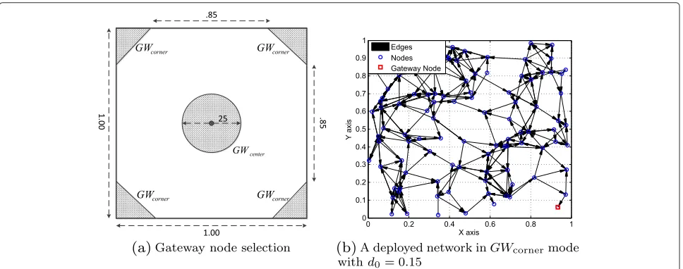
6.1 Network deployment and message generation To set up the simulations, we generate random deploy-ments of networks with directed links, obtained from a transmission power loss model. Specifically, a certain number of nodes,n, are deployed in a unit square two-dimensional region, according to a uniform distribution. One of the deployed nodes in the network is randomly picked to be the gateway node,v0, in which the messages
are decoded. In our simulations, we examine two differ-ent probability models to pick the gateway node. In the first model, denoted by GWcorner, the gateway node is
uni-formly picked from the nodes within the region in the corners of the unit square, as shown in Figure 4a. In the second model, denoted by GWcenter, the gateway node is
uniformly picked from the nodes within the region in the center of a unit square, as shown in Figure 4a.
The asymmetric connectivity (which is different from full duplex transmission over links) of two nodes is deter-mined according to an exponential power decay model: if there is a distance between nodeiand nodej, denoteddi,j,
then there is an edge (link) fromitoj; if
di,j≤d0, (44)
and
Pi,j≤P0, (45)
where d0 is a threshold which determines the
commu-nication range of sensor nodes,Pi,j is a uniform random
variable between 0 and 1, and P0 (0 < P0 ≤ 1) tunes
the average percentage of nodes in the communication
range of a sensor toward which there will be a link. We change the value ofd0 (and typically keepP0 = 0.9) to generate networks with different number of edges and dif-ferent maximum hop distances, as described later in this section. Different settings for generating network deploy-ments, the resulting average degree of nodes|In(v)|, and the resulting average hop distances of nodes from the gateway node are presented in Table 1.
In our simulation, each communication link (edges) can maintain a lossless communication of 1 bit per use, i.e.,
Ce = 1, for alle ∈ E. We also assume that there is no
interference involved from transmission in other nodes which may have been achieved by using a time multiplex-ing strategy. A sample network deployment is shown in Figure 4b, where the arrows represent the directed links between the nodes.
To generate a realization of messages,x, we first gen-erate ak-sparse random vector,sk, whose non-zero com-ponents are uniformly distributed between−12 and+12. Then, a near-sparse vector,s, is obtained such that ele-ments of(s−sk)are drawn from independent zero-mean uniform random variables and
s−sk 1 s
1
=k. (46)
This is followed by generation of an orthonormal
ran-dom matrix, φ, and calculating random messages:x =
φ·s. To ensure thatxj’s are bounded, they are normalized
between−qmax and+qmax (xj’s are multiplied by a
con-stant value). The value ofqmax used for the simulations
does not affect the simulation results, since we are using average SNR as a measure of decoding quality. We study the performance of different transmission scenarios by
Table 1 Number of hops in each deployment setting with
n=100nodes
Simulation settings Average|In(v)| Average hops
d0=0.15, GWcorner 5.3 9.7
d0=0.15, GWcenter 5.3 5.3
d0=0.25, GWcorner 13.9 3.9
d0=0.25, GWcenter 13.9 2.3
d0=0.35, GWcorner 24.8 2.7
d0=0.35, GWcenter 24.8 1.7
repeating our simulations for different values of sparsity factor, kn, and near-sparsity parameter,k.
The average signal-to-noise ratio (SNR) is used as the quality measure in our numerical comparisons. Explicitly, for the decoded messages in a scheme,xˆ, the average SNR is defined as
SNR=20 log10 x
2 x− ˆx
2
, (47)
where()stands for the average over different realizations of network deployments. For each realization of network deployment, we only generate one realization of messages, and therefore, taking the average over different network deployments is enough to obtain the average SNR values.
The payback measure in our comparisons is the corre-sponding average delivery delay, to achieve the required quality of service (average SNR). Explicitly, delivery delay for a transmission which has terminated att is equal to (t−1)Lin all cases of transmission scenarios. In the case of packet forwarding, we do not consider the learning period required to find the routes from each sensor node to the decoder node.
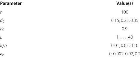
The used simulation parameters are listed in Table 2. In the table, we describe the different simulated transmission scenarios.
6.2 Quantized Network Coding
For each generated random network deployment, we
per-form QNC with1-min decoding. Local network coding
Table 2 The parameters of messages and the networks used in our simulations
Parameter Value(s)
n 100
d0 0.15, 0.25, 0.35
P0 0.9
L 1,. . ., 40
k/n 0.01, 0.05, 0.10
k 0, 0.002, 0.02, 0.2
coefficients,αe,v(t)’s andβe,e(t)’s, are generated
accord-ing to the conditions of Theorem 3, where σ0 = 0.25.
Edge quantizers,Qe()’s, have uniform characteristic with
a range of [−qmax,+qmax] and 2L intervals (sinceCe =
1, ∀e). Randomαe,v(2)’s andβe,e(t)’s can be generated in
a pseudo-random way, and therefore, only the generator seed needs to be transmitted to the decoder in a packet header.
At the decoder, the received measurements up to t,
ztot(t), are used to recover the original messages. Specif-ically, for a realization of messages,x, we definexˆQNC(t)
to be the recovered messages, using 1-min decoding,
according to (28). The convex optimization, involved in (28), is solved by using the open source implementation of disciplined convex programming [43]. Moreover, the net-work deployment is assumed to be known at the decoder in order to build uptot(t)matrices (the random
gener-ator seed is enough to regenerate local network coding coefficients). Although the exact sparsity of messages,k, does not need to be known for performing1-min
decod-ing, the sparsifying transform,φ, should be known. The block length,L, has to be known at the decoder to be able to calculate the level of the effective measurement noise, i.e.,rec(t)’s.
6.3 Quantization and packet forwarding
For each deployment, we also simulated a routing-based packet forwarding and compared it with the results for QNC. To find the routes from each node to the gate-way node, we find the shortest path from each node to the gateway node using the Dijkstra algorithm [44]. Fur-ther, the real-valued messages,xv’s, are quantized at their
corresponding source nodes, by using similar uniform quantizers, as used in QNC transmission. The system delivers allxv’s to the decoder node over a certain period
of time and keeps track of delivered messages over time,t, in the recovered vector of messages,xˆPF(t). Moreover, if a message,xv, is not delivered by time index,t, zero is used
as its recovered value:
{ˆxPF(t)}v=0. (48)
6.4 Quantization and packet forwarding with CS decoding
The quantization and packet forwarding with CS decod-ing (QandPFwithCS) scenario is exactly the same as the quantization and packet forwarding (QandPF) scenario, except at the decoder side. Specifically, at the decoder node, if the messages of some nodes are still not deliv-ered, the decoder tries to recover them from the other received (quantized) messages, using compressed sensing decoding. Explicitly, we definetot,PF(t) to be the
{tot.PF(t)}i,v=
1, Q(xv)delivered bytand corresponds toith received packet,
0, Q(xv)not delivered byt , (49)
andztot,PF(t)to be the set of received (delivered via PF) quantized messages at the decoder. In such case, the following1minimization is solved:
ˆ
quantized delivered messagesg. Then, for each v if its quantized messagesQ(xv) is still not delivered, we use {ˆxPFCS,0(t)}v, meaning
As it can be predicted, compressed sensing-based decoding tries to find an approximate estimation for the un-delivered messages by using the redundancy of mes-sages and improves the overall performance in terms of recovery error norm.
6.5 Quantization and network coding
Conventional finite field network coding is also simulated for transmission of messages to the decoder node. In this scenario, similar to packet forwarding, the messages are first quantized at their source nodes, by using a uniform quantizer. The quantizers have a range between −qmax
and+qmax, and their step size depends on the transmis-sion block length,L. Then, the quantized messages are transmitted to the decoder node by running a classical batch-based finite field network coding [7,8]. The field size in network coding is determined by the value ofL, and the network coding coefficients are picked randomly and uniformly from the field elements. At the decoder node, the received finite field packets are collected untiln
of them are stored, and the transmission is then stopped. If the finite field matrix, which maps the messages to the received packets at the decoder node, has full column rank, then the quantized messages can be reconstructed without any error. However, if the field size is not large enough and matrix inversion is not possible, then none of the messages can be decoded. In such case, we set the reconstructed (decoded) messages to be equal to their mean value (i.e., 0 in our simulations):
{ˆxQandNC(t)}v=0, ∀v. (52)
This is referred to as all or nothing decoding in the conventional network coding literature. Similar to QNC scenario, the network deployment is assumed to be known at the decode node, and the mapping matrix (from mes-sages to received packets) can be built up by only receiving the seed of pseudo-random generators.
6.6 Analysis of simulation results
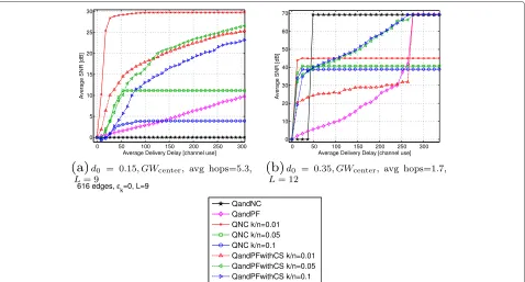
For a fixed block length,L = 9, the average SNR values versus the average delivery delay is depicted in Figure 5. In Figure 5a,b, the horizontal axis represents the prod-uct(t−1)L, which is the delivery delay, corresponding to
L = 9, for different values oft ≥ 1. The vertical axis is the average SNR, calculated according to (47), for QNC, QandPF (with and without compressed sensing decod-ing), and quantization and network coding (QandNC) scenarios.
As it is shown in Figure 5a,b, when using the same block length, QNC achieves significant improvement, compared to PF, for low values of delivery delay. These low delays correspond to the initialt’s in the transmission, at which a small number of packets are received at the decoder. As promised by the theory of compressed sens-ing, fewer measurements enable message recovery, with an associated measurement noise. After enough pack-ets are received at the decoder, QNC achieves its best performance (where the curve is almost flat). This best performance improves (i.e., average SNR increases) when the correlation of messages is higher (sparsity factork/n
is lower).
The best performance for QandPF, QandPFwithCS, and QandNC happens after a longer period of time than for QNC. As it can be seen, this is the best achievable qual-ity (SNR value), which is limited only by quantization noises at the source nodes, for both QandPF and QandNC scenarios. As it is also expected, using compressed sens-ing decodsens-ing (as in QandPFwithCS scenario) provides a better estimation of the messages before all the packets are delivered. Furthermore, as opposed to QandPF which shows a progressive improvement in the quality, QandNC has an all or nothing characteristic, as mentioned earlier. It is also interesting to note that low-density adjacency matrices in networks with small degree of nodes result in having (finite field) measurement matrices that are not of full rank in the QandNC scenario. Hence, as shown in Figure 5a, QandNC scheme fails to work properly.
Figure 5Average SNR versus average delivery delay for QNC, PF, and QandNC scenarios, whenk=0.(a)d0=0.15, GWcenter, average hops=5.3,L=9.(b)d0=0.35, GWcenter, average hops=1.7,L=12.
source quantization noise is involved). However, as it is shown in the following, QNC outperforms QandPF (with and without compressed sensing decoding) and QandNC scenarios in a wide range of delay values, when an appro-priate block length is chosen.
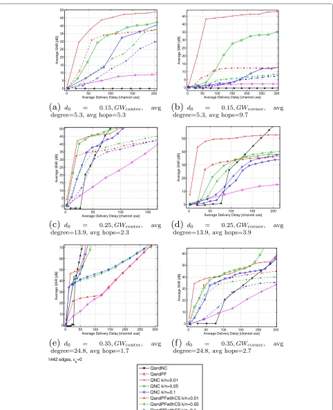
After simulating QNC, QandPF, QandPFwithCS, and QandNC scenarios for different block lengths and calcu-lating the corresponding delay and recovery error norms, we find the best values of block length for each specific average SNR value. The resultingL-optimized curves for each of these scenario are shown in Figure 6.
It can be seen in Figure 6a,b,c,d that, when the net-work does not have too many links (i.e., when the average hop distances are low), the proposed QNC scenario out-performs both routing-based packet forwarding (with and without compressed sensing decoding) and conventional QandNC scenarios. This is true for a wide range of average SNR values, varying up to around 35 dB, which is consid-ered as high quality in many applications. Moreover, as it is expected, the average SNR of QNC scenario increases when the correlation of messages increases (i.e., when the sparsity factor,k/n, decreases).
As shown in Figure 6e,f, when dealing with networks with very high number of edges, which results in small average hop distances, the proposed QNC scenario can-not outperform QandNC scenario, for very high SNR values (explicitly for average SNR values higher than 40 dB). This may be a result of quantization noise
pro-pagation through the network during the QNC steps, which strengthen the effective measurement noise above the level that sparse recovery can compensate.
By comparing the figures, in which only the loca-tion of gateway node has changed, i.e., from GWcenter
to GWcorner (Figure 6a to Figure 6b and Figure 6c to
Figure 6d), we can understand that QNC shows a more robust behavior than PF and QandNC schemes. In other words, QNC does not suffer from the complications (especially happening in packet forwarding) caused by asymmetric distribution of network flow. Using com-pressed sensing decoding for packet forwarding, as in QandPFwithCS scenario, improves the performance of packet forwarding in this situation, although it cannot outperform QNC scenario.
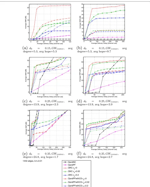
We have also studied the effect of the near-sparsity
parameter,k, on the performance of our QNC scheme.
Those results are shown in Figure 7, where the average SNR is depicted versus the average delivery delay, for dif-ferent settings of network deployment and a fixed sparsity factor ofk/n= 0.01. Increasing the near-sparsity param-eter, k, means that the generated messages are getting
further away from the sparsity model. As a result, the
performance of QNC degrades whenk increases, which
Figure 6Average SNR versus average delivery delay fork=0.(a)d0=0.15, GWcenter, average degree=5.3, average hops=5.3.(b)
Figure 7Average SNR versus average delivery delay fork/n=0.01.(a)d0=0.15, GWcenter, average degree=5.3, average hops=5.3.(b)
QNC scenario. We are currently studying such possibility, and our initial findings are reported in [45,46].
In the routing-based packet forwarding scenarios (with and without compressed sensing decoding), the interme-diate (sensor) nodes have to go through route training and queuing of packets. One of the main advantages of QNC is that the intermediate nodes should only carry out simple linear combination and quantization, which reduces the required computational power of interme-diate sensor nodes (they still have to perform sensing and physical layer transmission). On the other hand,
at the decoder sides, QNC requires an 1-min decoder
which is potentially more complex than the receiver required for packet forwarding. However, since the gate-way node is usually capable of handling higher compu-tational operations, this may not be an issue in practical cases.
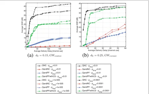
6.7 QNC in lossy networks
Although it is not the main focus of our paper, we have run some numerical simulations to assess the robustness of QNC scenario in lossy networks. Specifically, we consider a network model similar to the one used for the lossless case, but with the presence of packet losses. More pre-cisely, all the links are assumed to have a bit dropping rate
ofpdrop, i.e., a bit (which corresponds to a symbol in the
case ofC0= 1 considered in the simulations) is dropped (lost) during the transmission with a probability ofpdrop.
When dealing with packets of lengthL, a packet is consid-ered as being dropped if one or more of its bits are lost. This will be applied to all different transmission schemes, described in Section 6.1.
During the packet forwarding, if a packet is not suc-cessfully transmitted over a channel, it needs to be re-transmitted completely. Moreover, in the QandNC and QNC scenarios where finite field network coding and Quantized Network Coding are adopted, loss of a packet (transmitted over a link) is reflected by a zero value for the corresponding local network coding coefficient.
The simulation results for this lossy network scenario are shown in Figure 8. Similar to the case of lossless net-work, the curves are obtained by finding the appropriate packet length for each SNR value. We have used a wide range of bit loss ratespdropfor our simulations and shown results for a few representative values ofpdrop. Specifically,
we present the performance curves for a low loss rate of
pdrop=10−5, 10−4and a high loss rate ofpdrop=10−2.
Since the low SNR values (low decoding quality) in QNC scenario are obtained by using small packet lengths (small values ofL), the probability of having a bit drop in
(a)
(b)
the packet is smaller, compared to a larger packet length (largerL). As a result, the resulting performance curves are not very different, when having different loss rates. This is shown in Figure 8a,b, where there is a small gap between the curves of differentpdrop values at low SNR values.
Moreover, since the compressed sensing decoder exploits the correlation between the messages, it is able to reconstruct some messages when their corresponding lin-ear measurements are lost in the transmission. This fact can also be seen in QandPF scenario when compressed sensing decoding is adopted.
7 Conclusions
Joint source network coding of correlated sources was studied with a sparse recovery perspective. In order to achieve encoding of correlated sources without requir-ing the encoders to know the source correlation model, we proposed Quantized Network Coding, which incorpo-rates real field network coding and quantization to take advantage of decoding using linear programming. Thanks to the work in the literature of compressed sensing, we discussed theoretical guarantees to ensure efficient encoding and robust decoding of messages. Moreover, we were able to make conclusive statements about the robust recovery of messages, when fewer number of received packets than the number of source signals (messages) were available at the decoder. Finally, our computer simu-lations verified the reduction in the average delivery delay, by using Quantized Network Coding.
Currently, we are studying the feasibility of near mini-mum mean squared error decoding, when other forms of prior information are available about the source. Specif-ically, we have suggested the use of belief propagation-based decoding [45] in a Bayesian scenario. However, more theoretical work is needed to derive mathematical guarantees for robust recovery. Studying the general case of lossy networks with interference between the links is also one of the proposed future directions.
Endnotes
aThey only mention that dense networks satisfy
restricted eigenvalue condition and do not prove it.
bAlthough the impact and value ofLare not discussed
at this point, it is an important design parameter, which will be extensively discussed in Section 6.
cIn this paper, all the vectors are column-wise.
dThis choice reduces the tail probabilities defined later
on in Equation 26 and, as such, increases the probability of the measurement matrix satisfying RIP.
eExplicitly, we have a predetermined set of orthogonal
matrices, used asβe,e(t)’s. Further, the variance of
αe,v(2)’s are picked the same such that the mean of
2-norms (defined in [32]) is equal to 1.
fAlthough a uniform quantizer may not be the best
choice for some message distributions, it is still widely used in practice. It also allows us to simplify the
mathematical analysis to provide a theoretical bound on the resulting recovery error. The study of the impact of different quantizer designs is left as a future work.
gThis depends on the characteristic of quantizers used
at the source node to quantize each message before packet forwarding. Specifically, in our simulations where we used uniform quantizers with step sizeQ,rec,PF(t)
is equal to the product ofQand the number of
delivered quantized messages.
Competing interests
The authors declare that they have no competing interests.
Acknowledgements
This work was supported by Hydro-Québec, the Natural Sciences and Engineering Research Council of Canada, and McGill University in the framework of the NSERC/Hydro-Québec/McGill Industrial Research Chair in Interactive Information Infrastructure for the Power Grid.
Received: 1 October 2013 Accepted: 18 February 2014 Published: 13 March 2014
References
1. I Akyildiz, W Su, Y Sankarasubramaniam, E Cayirci, A survey on sensor networks. IEEE Commun. Mag.40(8), 102–114 (2002)
2. C Chong, S Kumar, Sensor networks: evolution, opportunities, and challenges. Proc. IEEE.91(8), 1247–1256 (2003)
3. R Ahlswede, N Cai, S-Y Li, R Yeung, Network information flow. IEEE Trans. Inf. Theory.46, 1204–1216 (2000)
4. J Al-Karaki, A Kamal, Routing techniques in wireless sensor networks: a survey. IEEE Wireless Commun.11(6), 6–28 (2004)
5. T Ho, R Koetter, M Medard, D Karger, M Effros, The benefits of coding over routing in a randomized setting, inIEEE International Symposium on Information Theory,29 June–4 July 2003 (IEEE, Piscataway, 2003), p. 442 6. C Fragouli, Network coding for sensor networks, inHandbook Array
Processing Sensor Networks(Wiley Online Library, 2009), pp. 645–667 7. R Koetter, M Médard, An algebraic approach to network coding.
IEEE Trans. Netw.11(5), 782–795 (2003)
8. T Ho, M Medard, R Koetter, D Karger, M Effros, J Shi, B Leong, A random linear network coding approach to multicast. IEEE Trans. Inf. Theory.52, 4413–4430 (2006)
9. S Lim, Y Kim, A El Gamal, S Chung, Noisy network coding. IEEE Trans. Inf. Theory.57(5), 3132–3152 (2011)
10. A Dana, R Gowaikar, R Palanki, B Hassibi, M Effros, Capacity of wireless erasure networks. IEEE Trans. Inf. Theory.52, 789–804 (2006) 11. D Slepian, J Wolf, Noiseless coding of correlated information sources.
IEEE Trans. Inf. Theory.19(4), 471–480 (1973)
12. Z Xiong, A Liveris, S Cheng, Distributed source coding for sensor networks. IEEE Signal Process. Mag.21(5), 80–94 (2004)
13. TS Han, Slepian-wolf-cover theorem for networks of channels. Inf. Control. 47(1), 67–83 (1980)
14. T Ho, M Médard, M Effros, R Koetter, D Karger, Network coding for correlated sources, inProceedings of Conference on Information Sciences and Systems(CiteSeer, 2004)
15. A Ramamoorthy, K Jain, PA Chou, M Effros, Separating distributed source coding from network coding. IEEE Trans. Netw.14, 2785–2795 (2006) 16. Y Wu, V Stankovic, Z Xiong, S Kung, On practical design for joint
distributed source and network coding. IEEE Trans. Inf. Theory.55(4), 1709–1720 (2009)
17. G Maierbacher, J Barros, M Médard, Practical source-network decoding, in
6th International Symposium on Wireless Communication Systems(IEEE, Piscataway, 2009), pp. 283–287
19. F Kschischang, B Frey, H Loeliger, Factor graphs and the sum-product algorithm. IEEE Trans. Inf. Theory.47(2), 498–519 (2001)
20. D Donoho, Compressed sensing. IEEE Trans. Inf. Theory.52, 1289–1306 (2006)
21. R Baraniuk, M Davenport, M Duarte, C Hegde,An Introduction to Compressive Sensing(Addison-Wesley, Boston, 2011)
22. J Haupt, W Bajwa, M Rabbat, R Nowak, Compressed sensing for networked data. IEEE Signal Process. Mag.25, 92–101 (2008) 23. N Nguyen, D Jones, S Krishnamurthy, Netcompress: coupling network
coding and compressed sensing for efficient data communication in wireless sensor networks, in2010 IEEE Workshop on Signal Processing Systems,Oct 2010 (IEEE, Piscataway, 2010), pp. 356–361
24. C Luo, F Wu, J Sun, CW Chen, Compressive data gathering for large-scale wireless sensor networks, inProceedings of the 15th Annual International Conference on Mobile Computing and Networking,MobiCom ’09, (ACM, New York, 2009), pp. 145–156
25. S Feizi, M Médard, M Effros, Compressive sensing over networks, in48th Annual Allerton Conference on Communication, Control, and Computing
(IEEE, Piscataway, 2010), pp. 1129–1136
26. W Xu, E Mallada, A Tang, Compressive sensing over graphs, inIEEE International Conference on Computer Communications (INFOCOM)
(IEEE, Piscataway, 2011), pp. 2087–2095
27. M Wang, W Xu, E Mallada, A Tang, Sparse recovery with graph constraints: fundamental limits and measurement construction, inIEEE International Conference on Computer Communications (INFOCOM)(IEEE, Piscataway, 2012), pp. 1871–1879
28. S Feizi, M Medard, A power efficient sensing/communication scheme: joint source-channel-network coding by using compressive sensing, in
49th Annual Allerton Conference on Communication, Control, and Computing(IEEE, Piscataway, 2011), pp. 1048–1054
29. F Bassi, L Chao, L Iwaza, M Kieffer, Compressive linear network coding for efficient data collection in wireless sensor networks, inProceedings of the 2012 European Signal Processing Conference(IEEE, Piscataway, 2012), pp. 1–5
30. B Dey, S Katti, S Jaggi, D Katabi, M Medard, S Shintre, “Real” and “complex” network codes: promises and challenges, inFourth Workshop on Network Coding, Theory and Applications. 2008 NetCod 2008(IEEE, Piscataway, 2008), pp. 1–6
31. M Nabaee, F Labeau, Quantized network coding for sparse messages, in
IEEE Statistical Signal Processing Workshop,Ann Arbor, Aug 2012 (IEEE, Piscataway, 2012), pp. 832–835
32. M Nabaee, F Labeau, Restricted isometry property in quantized network coding of sparse messages, inIEEE Global Telecommunications Conference
Anaheim, Dec 2012 (IEEE, Piscataway, 2012)
33. EJ Candes, The restricted isometry property and its implications for compressed sensing. Comptes Rendus Mathematique.346(9-10), 589–592 (2008)
34. R Baraniuk, Compressive sensing. IEEE Signal Process. Mag.24(4), 118–121 (2007)
35. MF Duarte, S Sarvotham, MB Wakin, D Baron, RG Baraniuk, Joint sparsity models for distributed compressed sensing, inProceedings of the Workshop on Signal Processing with Adaptative Sparse Structured Representations(IEEE, Piscataway, 2005)
36. T Kailath,Linear Systems, vol. 1. (Prentice-Hall, Englewood Cliffs, 1980) 37. E Candes, J Romberg, Sparsity and incoherence in compressive sampling.
Inverse Probl.23(3), 969 (2007)
38. R Baraniuk, M Davenport, R Devore, M Wakin, A simple proof of the restricted isometry property for random matrices. Constr. Approx.28(3), 253–263 (2007)
39. E Candes, T Tao, Decoding by linear programming. IEEE Trans. Inf. Theory. 51, 4203–4215 (2005)
40. W Dai, HV Pham, O Milenkovic, Distortion-rate functions for quantized compressive sensing, inIEEE Information Theory Workshop on Networking and Information Theory(IEEE, Piscataway, 2009), pp. 171–175
41. A Zymnis, S Boyd, E Candes, Compressed sensing with quantized measurements. IEEE Signal Process. Lett.17(2), 149–152 (2010) 42. L Jacques, DK Hammond, JM Fadili, Dequantizing compressed sensing:
when oversampling and non-Gaussian constraints combine. IEEE Trans. Inf. Theory.57(1), 559–571 (2011)
43. M Grant, S Boyd, CVX: Matlab software for disciplined convex programming, version 1.21 (2012). http://cvxr.com/cvx. Accessed Aug 2012
44. E Dijkstra, A note on two problems in connexion with graphs. Numerische Mathematik.1(1), 269–271 (1959)
45. M Nabaee, F Labeau, Non-adaptive distributed compression in networks, in2013 IEEE Digital Signal Processing and Signal Processing Education Meeting (DSP/SPE)(IEEE, Piscataway, 2013), pp. 239–244
46. M Nabaee, F Labeau, Bayesian quantized network coding via generalized approximate message passing, in2014 Wireless Telecommunications SymposiumWashington, DC Apr 2014 (IEEE, Piscataway, 2014)
doi:10.1186/1687-1499-2014-40
Cite this article as:Nabaee and Labeau:Quantized Network Coding for correlated sources.EURASIP Journal on Wireless Communications and Network-ing20142014:40.
Submit your manuscript to a
journal and benefi t from:
7 Convenient online submission 7 Rigorous peer review
7 Immediate publication on acceptance 7 Open access: articles freely available online 7 High visibility within the fi eld
7 Retaining the copyright to your article