Reliability analysis of subway vehicles based on the data of operational failures

(1)

R E S E A R C H

Open Access

Reliability analysis of subway vehicles

based on the data of operational failures

Huaixian Yin

1,2*

, Kai Wang

3

, Yong Qin

1

, Qingsong Hua

2

and Qibin Jiang

3

Abstract

A large quantity of failure data for subway vehicles was collected from long-term field investigations and technical exchanged. These failure data has a guiding significance for preserving subway system. By preprocessing (screening, refining, and classification) the original data and statistical analysis, we establish some selected model, then we use A-D test to verify the degree of fitting in selected model so that we can determine the optimal failure distribution model, and then the reliability characteristic quantities could be calculated by the optimal failure distribution model. These reliability characteristic quantities can predict failure rate, failure number, etc. It can be used to assist proper maintenance scheduling to reduce the occurrence of accidents and significant to important practical guiding.

Keywords:Reliability analysis, Survival analysis, Parameter estimate, Degree of fitting

1 Introduction

Since the first subway line was put into operation in October 1969, there are more than 20 cities owned their subway systems in China, with a total operating mileage over 2400 km. Chinese subway companies have accumu-lated large amounts of failure data up to now, these data truly reflect field operating conditions. However, there are certain shortcomings in the data, much of it does not comply with uniform standards or is derived from complex data resources, and it may be missing import-ant information [1, 2]. A large-scale subway system in China requires the successful prevention of major acci-dents and sudden incident; otherwise, catastrophic results might occur. Therefore, how to analyze and deal with such complex large-scale operation failure data, to ensure the safety of urban rail transit has become a major research topic in the field of subway reliability research.

Wang et al. presented the service life estimation method based on the three-parameter Weibull max-imum likelihood estimation, respecting to the compo-nent wearing of high speed multiple units [3]. A new product data management method was created in [4] to process the component maintenance and historical

failure data of electric multiple units, which resulted in a 30% increase in the reliability. Others performed the re-liability analysis in [5] for the Bogie system of Sweden’s railways based on data collected by a wireless sensor net-work. The problem with this method was that the uncer-tainty in the time domain was not considered. In [6], they adopted the random process and reliability theory to investigate the failure distribution rules and reliability of rail vehicle components [6]. Yu et al. deduced the safety domain curve of high-speed trains through deducting the extreme sensitivity of system reliability [7]. Some articles used the nonparametric method to esti-mate the reliability function of the mechanism under ex-treme impact [8, 9], and Jiang analyzed the application of the proportional risk function in a repairable system [10].

The existing failure-data-based reliability analyses were mainly focused on railway passenger and freight vehicles and high-speed train. However, little analyses attention has been paid to the subway system. In essence, the subway is different from the railway in various aspects, such as the departure intervals, operating cycle, line conditions, the failure position, frequency, and mainten-ance data.

Parameter estimation method of reliability can only be used in known lifetime distribution. Unknown distribu-tion usually uses probabilistic paper graph method and similar WPP graphic estimation method to study the distribution; these methods need to draw the curve of

* Correspondence:[email protected]

1

School of Traffic and Transportation, Beijing Jiaotong University, No. 3 Shang Yuan Cun, Hai Dian District, Beijing 100044, China

2_{College of Mechanical and Electrical Engineering, Qingdao University,}

Qingdao 266071, China

Full list of author information is available at the end of the article

(2)

reliability and failure time. By further studying the shape of the curve, the reliability model of the failure data is determined. If the distribution model of a group failure data is not known, survival analysis theory can assume the group failure data conforms to all models, then each distribution model is fitted and the best fitting distribu-tion model is selected, Finally, the parameter estimadistribu-tion and hypothesis testing are carried out. Survival analysis method can effectively solve uncertain failure time inter-val problems under the mechanism of censored data on subway vehicles, in order to get more reasonable results of reliability analysis. Therefore, we used survival ana-lysis technology to perform the reliability anaana-lysis of the subway vehicles for the purpose of accurately grasping the working status of key subway systems, including identifying failures, performing maintenance, and securing the subway’s operation. The survival analysis method has particular advantages in the processing and analysis of censored data during the application of non-parametric, parametric, and semi-parametric survival analysis.

2 Fault distribution model and methods analysis 2.1 Survival analysis

Survival analysis is a technology of statistical analysis about survival time. Based on data collected via experi-ment or survey, it statistically analyzes the survival time of living creatures, human, or other things with a sur-vival cycle and represents the results in the form of a survival function, probability density function, danger scale function, and average life [11, 12].

2.1.1 Survival function

Survival function which is also called reliability function is defined as

RðtjÞ ¼SðtjÞ ¼PðT >tjÞ ¼1−PðT≤tjÞ

¼1−FðtjÞ ð1Þ

On the equation,R(tj) is reliability function andS(tj) is survival function. The probability that the individual fail-ure intervalTis greater thantj, which has the following properties R(0) = 1 and R(∞) = 1. F(tj) is unreliability function. It indicates the probability that product is unable to complete the function under the specified time and conditions.F(tj) is the distribution function ofT[13].

FðtjÞ ¼PðT≤tjÞ ¼nðtÞ

N ;0≤t≤∞ ð2Þ

On the equation,Nis the product sample andn(t) are the numbers of failure at samples time.

2.1.2 Probability density function

Probability density function p(tj) is the ratio of the failure numbersDjand the total observation numbersN that during the periodtj−1totj.

pðtjÞ ¼fðtjÞ ¼pðT ¼tjÞ ¼Dj

N;1≤j≤n ð3Þ

2.1.3 Danger scale function

Danger scale functionλ(tj) represents the instantaneous failure rate of the observing objects at the moment tj which is not failure at the momenttj−1. It is also called damage function and the failure rate function. It is used to measure whether an individual is prone to fail at some time [14].

λ tj ¼P T ¼tjjT≥tj¼p tj = S_{ð Þ}_t_j₋₁

h i

ð4Þ

On the equation, there is the following relationship

SðtjÞ ¼Y_t

i≤t½1−λðtjÞ ð5Þ

2.1.4 Average life

Average life means trouble-free working time of product. For repairable products, average life is the mean operat-ing time between failures [15].

u¼EðtÞ ¼Xn_j_¼₁SðtjÞðtj−tj−1Þ ð6Þ

2.2 Model building and methods

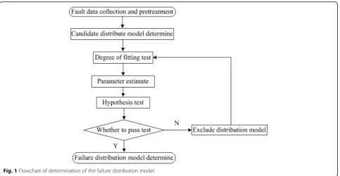
Figure 1 shows a flowchart of reliability analysis via the determination of failure distribution model using sur-vival analysis theory.

2.2.1 Fault data collection and pretreatment

In terms of fault data collection and pretreatment, we use statistics method, eliminate or merge the fault entry, and eventually determine the effective subway vehicles failure data.

2.2.2 Candidate distributions

A large number of articles were reviewed to determine the candidate distributions, including the exponential distri-bution, logarithmic normal distridistri-bution, two-parameter Weibull distribution, and three-parameter Weibull distri-bution [16].

2.2.3 The maximum likelihood estimation

The maximum likelihood estimation method was used in this study for the parameter estimation of the optimal distribution. The basic principle of this method is as fol-lows: assuming the known population distribution and

(3)

an unknown parameterθ, one valueθbis chosen from all possible values, which can result in the maximal prob-ability of the observed results. θbis then defined as the maximum likelihood estimation value of θ, and the parameter estimation method was named as maximum likelihood estimation method [17].

X1, X2,…, Xn are samples from the X, thus the joint density ofX1,X2,…,Xnis

Y_n

i¼1fðxi;θÞ ð7Þ

x1, x2,…, xn is a sample value corresponding to the sampleX1,X2,…,Xn, the function is

LðθÞ ¼Lðx1;x2;⋯;xn;θÞ ¼

Y_n

i¼1fðxi;θÞ ð8Þ

L(θ) is called the likelihood function of the sample. If

Lðx1;x2;⋯;xn;θbÞ ¼ maxθ∈ΘLðx1;x2;⋯;xn;θÞ ð9Þ

The θbðx1;x2;⋯;xnÞ is called the maximum likelihood

estimation ofθ.

Thus, the problem to determine the maximum likeli-hood estimation is attributed to seek the maximum in the differential calculus problem.

In many cases,f(xi, θ) is differentiable onθ, θbserved from the equation

d

dθLðθÞ ¼0 ð10Þ

2.2.4 Degree of fitting

For the degree of fitting and hypothesis testing in the candi-date model, Minitab software was used to perform the A-D (Anderson-Darling) test to verify the effectiveness of the models. The statistics from the A-D test can be used to compare the fitting condition of several distributions, thereby identifying the optimal distribution. In engineering practice, the A-D test statistical variableA2 can be calcu-lated from common discrete expressions (11). Specifically, it is the weighted square distance between data points and the fitting curve. The closer to the end of distribution the point is, the bigger the weight becomes [18, 19]. Hence, a smallA2 represents a higher degree of fitting, the expres-sion is:

A2_¼_−n−1 n

Xn

i¼1ð2i−1Þ ln

F xð Þi þ _lnð1−F xðn−iþ1ÞÞ

h i

ð11Þ

On the equation,n is the sample size andF(xi) is the empirical cumulative distribution function obeying to the normal distribution.

F xið Þ ¼ϕ xi_σ−x

ð12Þ

First, the p values of the four candidate distributions were compared. If p> 0.05, it indicated that the corre-sponding distribution was able to fit the failure data. The distributions with good fitting results were preserved, and then the A-D statistical variable was calculated. The

(4)

distribution with a minimum A-D value was chosen as the optimal distribution model.

3 Example analysis and results 3.1 Fault data statistics

The structure of subway vehicles includes the running gear, traction system, brake system, control and diagnostic system, and the auxiliary system. All of these subsystems play a significant role in the vehicle’s reliability and safe operation. There are frequent subway failures and accidents due to the rapid development of the urban subway transportation system. Therefore, we investigated the reliability of the key subsystems in sub-way vehicles in this study.

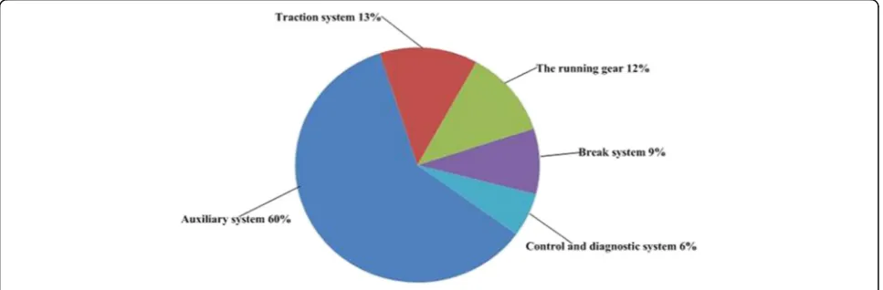
The original data of operational failures covered the above five systems were screened and calculated statisti-cally, including a total of 8000 entries from January 2009 to December 2013. Each failure was recorded with its number, date of occurrence, vehicle number, failure de-scription, and failure consequences. Figure 2 shows the statistics of the annual failures about each subsystem,

vehicle door system, the illumination system, and other incorporate into the auxiliary system. Figure 3 shows the statistics of the data. By sorting the data based on the number of failures, we found that most failures were related to the auxiliary systems, followed by the traction system, running gear, braking system, and control and diagnostic systems.

Because most of the subway vehicles system life distribu-tion data is censored data, we use the survival analysis in the system time between failures to process censored data. In the fault data statistics, censored data mainly includes two categories. One kind is interval-censored data, if the maintenance work is reliable and the failure occurs between the overhaul and the last overhaul, so fault time is an inter-val, uncertain value, and fault specific time unknown. One kind is the right censored data, statistical period of the be-ginning and the end will have censored data, and fault time is greater than a certain value of tracked. We use common failure distribution function on censored data for maximum likelihood method of parameter estimation to calculate A-D statistics to select fitting of better distribution function.

Fig. 3Statistics of the operational failure of subway key components

Fig. 2Annual fault distribution diagram of key system

(5)

3.2 Result and discussion

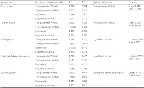
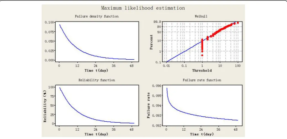
Based on the screened data, the operating time between failures was calculated and imported into Minitab [20, 21]. The “Reliability/Survival Statistics” tool was used to perform the maximum likelihood estimation for four

candidate distributions (the exponential distribution, logarithmic normal distribution, two-parameter Weibull distribution, and three-parameter Weibull distribution). Figure 4 shows the fitting graph of the service life distribu-tion for tracdistribu-tion system. Table 1 presents the p value,

Table 1Fault distribution fit test table of the key subsystems

Subsystems Candidate distribution model P A-D Optimal distribution Parameter

Running gear Two-parameter Weibull 0.249 0.704 Two-parameter Weibull Shape 0.9124

Scale 13.5450

Three-parameter Weibull 0.007 1.325

Exponential 0.253 0.921

Logarithmic normal 0.097 0.876

Traction system Two-parameter Weibull 0.086 1.380 Two-parameter Weibull Shape 0.9940

Scale 10.6495

Three-parameter Weibull < 0.005 5.463

Brake system Two-parameter Weibull 0.014 1.120 Logarithmic normal Location 2.3693

Scale 1.3003

Exponential < 0.003 3.376

Control and diagnostic system Two-parameter Weibull 0.242 0.672 Logarithmic normal Location 2.5573

Scale 1.3581

Auxiliary system Two-parameter Weibull 0.096 1.974 Logarithmic normal distribution Location 1.4915

Scale 0.9349

Three-parameter Weibull <0.005 4.060

(6)

A-D statistical variable, screen for the optimal distribu-tion, and parameter estimation obtained from the max-imum likelihood estimation method.

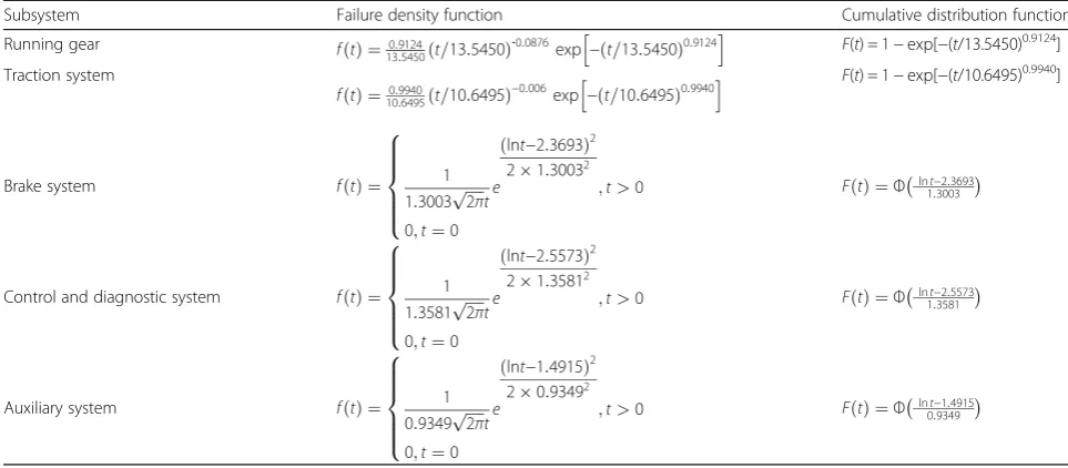
The parameter value of the maximum likelihood estimation that meets the distribution of the operating time between failures in Table 1; every subsystem was substituted into the reliability characteristic functions of the optimal distribution, thereby allowing for the derivation of the reliability characteristic functions of each subsystem (failure density function, cumulative dis-tribution function, reliability function, and failure rate function). The mean time between failures was based on the operating time between failures; it was calculated and is shown in Tables 2 and 3. Similarly, the graph of the reliability characteristic function of traction system was plotted, as shown in Fig. 5.

Tables 2 and 3 shows that the mean operating time be-tween failures for the running gear, traction system, brake system, control and diagnostic system, and auxil-iary systems was 14, 11, 25, 32, and 7 days. The mean operating time between failures, namely, the failure rate,

increased in the following order: auxiliary systems, trac-tion system, running gear, brake system, and control and diagnostic systems. These results are consistent with the number of failures collected from the field data.

The reliability characteristic function model can be used to predict various reliability characteristics, such as the reliability, unreliability, and the mean time between failures. In addition, the subway system can reduce the occurrence of incidents by mean of vehicle maintenance schedules according to the characteristic variables. For example, assuming that the reliability of the running gear of a subway vehicle should be above 95%, R(t) = 0.95 was substituted into the reliability characteristic function of the running gear in Tables 2 and 3. We can get the formula as follows:

t¼13:5450 ln 1

Table 3The reliability characteristic functions of each subsystem

Subsystem Reliability function Failure rate function Average life (days)

Running gear R(t) = exp[−(t/13.5450)0.9124_] _λ_{ð Þ ¼}_t 0:9124

Table 2The reliability characteristic functions of each subsystem

Subsystem Failure density function Cumulative distribution function

Running gear _{f t}_{ð Þ ¼}0:9124

(7)

λð Þ ¼t 0:9124

13:5450

t₌

13:5450

ð Þ−0:0876

¼0:0896 ð15Þ

It can be concluded that maintenance should be scheduled every other day in order to meet the reliability requirements of the running gear. Similarly, the main-tenance plan for the other subsystem can be formulated.

4 Conclusions

Based on the operational failure data of subway vehicles, a reliability analysis method of subway subsystems was developed based on the survival analysis theory. By fil-tering, classification, and the preprocessing of the failure data, the numbers of failure and mean operating time between failures were obtained for each subsystem. The results showed that the failure rate increased in the fol-lowing order: auxiliary systems, traction system, running gear, brake system, and control and diagnostic systems. The optimal failure distribution model of every subsys-tem was determined by the use of Minitab. We can for-mulate the vehicle maintenance schedule to direct our daily maintenance work, which could observably reduce the failure of subsystem.

The reliability characteristic functions can be used to obtain a scientific estimation of the reliability character-istic variables. As the rapid construction and increasingly complex of domestic subway system, reliability charac-teristic function for future subway has guiding signifi-cance to the construction and systemic maintenance. In

the future, reliability analysis of the subway will get widespread attention and long-term development.

Due to the limitation of time and ability, this article only focuses on the subject of each subsystem. We will analyze the reliability of the specific components to find fault specific reason and provide guidance for train maintenance to reduce the incidence of failure.

Acknowledgements

We thank the reviewers for their detailed reviews and constructive comments which have helped to improve the quality of this article.

Funding

This work has been supported by National Key Technology Research and Development Program (2015BAG12B01).

Authors_’contributions

HY gave the original ideas and wrote the manuscript. KW and QJ participated in the establishment of simulation model. YQ and QH provided failure data and analyses. All authors read and approved the final manuscript.

Competing interests

The authors declare that they have no competing interests.

Publisher’s Note

Springer Nature remains neutral with regard to jurisdictional claims in published maps and institutional affiliations.

Author details

1_{School of Traffic and Transportation, Beijing Jiaotong University, No. 3}

Shang Yuan Cun, Hai Dian District, Beijing 100044, China.2College of Mechanical and Electrical Engineering, Qingdao University, Qingdao 266071, China.3_{College of Automation and Electrical Engineering, Qingdao}

(8)

Received: 4 August 2017 Accepted: 23 November 2017

References

1. S Derrible, C Kennedy, The complexity and robustness of metro networks. Physica A389(17), 3678_–3691 (2010)

2. Y Hamdouch, HW Ho, A Sumalee, G Wang, Schedule-based transit assignment model with vehicle capacity and seat availability. Transp. Res. Pt. B-Methodol.45(10), 1805–1830 (2011)

3. D Cousineau, Fitting the three-parameter Weibull distribution: review and evaluation of existing and new methods. IEEE Trns. Dielectr. Electr. Insul.

16(1), 281–288 (2009)

4. MT Huynh, A Hopkins, R Norris, The completeness and reliability of threshold and false-discovery rate source extraction algorithms for compact continuum sources. Publ. Astron. Soc. Aust.29(3), 229–243 (2012) 5. M Gholami, RW Brennan, Comparing two clustering-based techniques to

track mobile nodes in industrial wireless sensor networks. J. Syst. Sci. Syst. Eng.25(2), 177_–209 (2016)

6. JH Kim, JW Jin, JH Lee, Failure analysis for vibration-based energy harvester utilized in high-speed railroad vehicle. Eng. Fail. Anal.73, 85–96 (2017) 7. S Giappino, D Rocchi, P Schito, Cross wind and rollover risk on lightweight

railway vehicles. J. Wind Eng. Ind. Aerodyn.153, 106_–112 (2016) 8. Z Ye, LC Tang, H Xu, A distribution-based systems reliability model under

extreme shocks and natural degradation. IEEE Trans. Reliab.60(1), 246–256 (2011) 9. AA Shabana, JR Sany, A survey of rail vehicle track simulations and flexible

multibody dynamics. Nonlinear Dyn.26(2), 179_–212 (2001)

10. S-T Jiang, TL Landers, TR Rhoads, Assessment of repairable-system reliability using proportional intensity models: a review. IEEE Trans. Reliab.

55(2), 328–336 (2006)

11. F Shi, Z Zhou, J Yao, H Huang, Incorporating transfer reliability into equilibrium analysis of railway passenger flow [J]. Eur. J. Oper. Res.

220(2), 378–385 (2012)

12. MK Ardakani, L Sun, Decremental algorithm for adaptive routing incorporating traveler information. Comput. Oper. Res.39(12), 3012_–3020 (2012)

13. Y(M) Niea, X Wua, JF Dillenburgb, PC Nelsonb, Reliable route guidance: a case study from Chicago. Transp. Res. Pt. A-Policy Pract46(2), 403–419 (2012) 14. D Canca, A Zarzo, PL González-R, A methodology for schedule-based paths

recommendation in multimodal public transportation networks. J. Adv. Transp.47(3), 319–335 (2013)

15. K Wang, L Li, T Zhang, et al., Nitrogen-doped graphene for supercapacitor with long-term electrochemical stability. Energy70, 612–617 (2014) 16. LijunTian, H Huang, T Liu, Day-to-day route choice decision simulation

based on dynamic feedback information. J. Transp. Syst. Eng. Inform. Technol10(4), 79–85 (2010)

17. ECG Wille, E Yabcznski, HS Lopes, Discrete capacity assignment in IP networks using particle swarm optimization. Appl. Math. Comput.

217(12), 5338–5346 (2011)

18. A Sedeño-Noda, An efficient time and space K point-to-point shortest simple paths algorithm. Appl. Math. Comput.218(20), 10244–10257 (2012) 19. G Koulinas, L Kotsikas, K Anagnostopoulos, A particle swarm optimization

based hyper-heuristic algorithm for the classic resource constrained project scheduling problem. Inf. Sci.277, 680–693 (2014)

20. K Wang, L Li, H Yin, et al., Thermal modelling analysis of spiral wound supercapacitor under constant-current cycling. PLoS One10(10), e0138672 (2015) 21. Tian Z.G, Wong L, Safaei N, A neural network approach for remaining useful

life prediction utilizing both failure and suspension histories. Mechanical Systems and Signal Processing.24, 1542–1555 (2010)