Numerical Solution of Nonlinear System of Partial Differential Equations by the Laplace Decomposition Method and the Pade Approximation

(1)

Numerical Solution of Nonlinear System of Partial

Differential Equations by the Laplace Decomposition

Method and the Pade Approximation

Magdy Ahmed Mohamed1_{, Mohamed Shibl Torky}2 1_{Faculty of Science, Suez Canal University, Ismailia, Egypt}

2_{The High Institute of Administration and Computer, Port Said University, Port Said, Egypt} Email: dr_magdy_ahmed53@yahoo.com, mohamedtorky@himc.psu.edu.eg

Received March 7, 2013; revised April 28, 2013; accepted May 9, 2013

Copyright © 2013 Magdy Ahmed Mohamed, Mohamed Shibl Torky. This is an open access article distributed under the Creative Commons Attribution License, which permits unrestricted use, distribution, and reproduction in any medium, provided the original work is properly cited.

ABSTRACT

In this paper, Laplace decomposition method (LDM) and Pade approximant are employed to find approximate solutions for the Whitham-Broer-Kaup shallow water model, the coupled nonlinear reaction diffusion equations and the system of Hirota-Satsuma coupled KdV. In addition, the results obtained from Laplace decomposition method (LDM) and Pade approximant are compared with corresponding exact analytical solutions.

Keywords: Nonlinear System of Partial Differential Equations; The Laplace Decomposition Method; The Pade Approximation; The Coupled System of the Approximate Equations for Long Water Waves; The Whitham Broer Kaup Shallow Water Model; The System of Hirota-Satsuma Coupled KdV

1. Introduction

The Laplace decomposition method (LDM) is one of the efficient analytical techniques to solve linear and nonlinear equations [1-3]. LDM is free of any small or large parameters and has advantages over other approximation techniques like perturbation. Unlike other analytical techniques, LDM requires no discretization and linearization. Therefore, results obtained by LDM are more efficient and realistic. This method has been used to obtain approximate solutions of a class of nonlinear ordinary and partial differential equations [1-4]. See for example, the Duffing equation [4] and the Klein-Gordon equation [3]. In this paper, the LDM is applied to, the Whitham-Broer- Kaup shallow water model [5]

,

t x x xx

t x x xx x

u uu v u

v vu uv v u_xx



 

   

     (1) with exact solution are given in [5] as

 





 













2

1

2 2 2

2

2 2 2

1

ò

, 2 tanh ,

, 2

2 ò tanh ,

u x t k k x t

v x t k

k k

    

    

      

    

   

    x t 

(2)

and the coupled nonlinear reaction diffusion equations [6],

2 2

, ,

t xx x

u ku u v u v kv u v u  

  

   (3) with exact solution are given in [6] as

 

2

2 2

4

, 2 1 tanh ,

2

4 4

, 2 tanh

2 2 2

B c k

u x t k c t cx

B c k B c k

v x t k c t cx

k c

   

 _    _

 

 

 

  _  _

 ,

(4)

and thesystem of Hirota-Satsuma coupled KdV [7].

1

3 3 3

2

3 ,

t xxx x x x

t xxx x

u u uu vw wv

v v uv

w w uw

   

  

,

(5)

with exact solution are given in [7] as

 









 













 





2 2 2

2 2 2 2

0 2

1 1

0 1

1

, 2 2 tanh ,

2

4 4

, tanh

3 3

, tanh ,

u x t k k k x t

k c k k k

v x t k x t

c c

w x t c c k x t

 



   _  _

  

  _  _

,

(2)

we discuss how to solve Numerical solution of nonlinear system of parial differential equations by using LDM. The results of the present technique have close agreement with approximate solutions obtained with the help of the Adomian decomposition method [8].

2. Laplace Decomposition Method

 

,

 

,

i i i

U

1, 2, , ,

g x t R U N U i n

t

 _ _ _ _

  (7)

where U



u u1, , ,2 un



,

with initial condition

   

,0 ,

i i

u x f x (8)

the method consists of first applying the Laplace trans- formation to both sides of (7)

 

£ £ ,

£ , 1,

i

i i

U

g x t t

R U N U i n



 _{  } _

 

_ 

 

 _  _  2, , ,

(9)

using the formulas of the Laplace transform, we get

 

 

£ £ ,

£ , 1,

i i

s U f x g x t

R U N U i n

  _ _

 _  _  2, , ,

(10)

in the Laplace decomposition method we assume the solution as an infinite series, given as follows

,

n n

U U







(11) where the terms n are to be recursively computed.

Also the linear and nonlinear terms i and

is decomposed as an infinite series of Adomian polynomials (see [8,9]). Applying the inverse Laplace transform, finally we get

U

R

, 1, 2, ,

i

N i  n

 



 



1 1 £ £ , £ , i i i i

U f x g x t

s

R U N U i n

 

  _ _





 _  _{ } 1, 2, , ,

(12)

3. The Pade Approximant

Here we will investigate the construction of the Pade approximates [10] for the functions studied. The main advantage of Pade approximation over the Taylor series approximation is that the Taylor series approximation can exhibit oscillati which may produce an approximation error bound. Moreover, Taylor series approximations can never blow-up in a fin region. To overcome these demerits we use the Pade approximations. The

Pade approximation of a function is given by ratio of two polynomials. The coefficients of the polynomial in both the numerator and the denominator are determined using the coefficients in the Taylor series expansion of the function. The Pade approximation of a function, symbol- ized by [m/n], is a rational function defined by

2

0 1 2

2 1 2 , 1 m m n n a a x a x a x m

n b x b x b x

   

  

  _ _ _{ }

 



 (13)

where we considered b0 = 1, and the numerator and denominator have no common factors. In the LD-PA method we use the method of Pade approximation as an after- treatment method to the solution obtained by the Laplace decomposition method. This after-treatment method im- proves the accuracy of the proposed method.

4. Application

In this section, we demonstrate the analysis of our numerical methods by applying methods to the system of partial differential Equations (1), (3) and (5). A comparison of all methods is also given in the form of graphs and tables, presented here.

4.1. The Laplace Decomposition Method Exampe 1. The Whitham-Broer-Kaup model [5] To solve the system of Equation (1) by means of Laplace decomposition method, and for simplicity, we

take 1

1_, _2, _3, _1, _1, ₀ 2 k

   

 _ _ _ _ _ _ 

 

  , we con-

struct a correctional functional which reads

 

 





 

 





1 £ 0 1 £ , 1 £ 0 1 £ 3

x x xx

x x xx xxx

u u

s

uu v u s

v v

s

vu uv v u

s            , ,  (14)

we can define the Adomian polynomial as follows:

     

0 0 0

, ,

n n n

n i n i x n i n i x n i n i x

i i i

A u u _ B v u _ C u v

  













(15)

we define an iterative scheme

 





 





1 1 1 £ £ , 1

£ £ 3

n n nx nxx

n n n nxx nxxx

u A v u

s

v B C v u

(3)

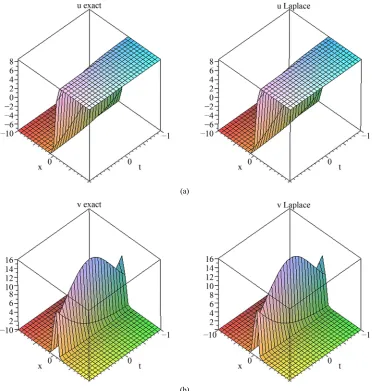
terms as Equation (18), and Figures 1(a) and (b) show the exact and numerical solution of system (1) with 16th terms by (LDM).

applying the inverse Laplace transform, finally we get Equations (17). Similarly, we can also find other components, and the approximate solution for calculating 16th

(a)

(b)

Figure 1. (a) Exact and numerical solution of u(x, t), −10 ≤x≤ 10, -1 ≤t≤ 1; (b) Exact and numerical solution of v (x, t), −10 ≤ x≤ 10, −1 ≤t≤ 1.

 





 





 





 

2

0 0 1 2 1 3

4 2

2 2

2 3 2 8 6 4 2

32 sinh 2

1 8

, 8 tanh 2 , , 16 16 tanh 2 , , , ,

2 cosh 2 cosh 2

16 8cosh 8cosh 1

8 sinh 2

, , , ,

cosh 2 1 16 cosh 32 cosh 24 cosh 8cosh

t x

t

u x t x v x t x u x t v x t

x x

t x x

t x

u x t v x t

x x x x x

        

 

  

   

,

(17)

 









 





 

4 2

3 2

2 3 8

4 2

2 2

3 4

8 8cosh 8cosh 1

8 sinh 2

1 8

, 8 tanh 2

2 cosh 2 cosh 2 3(1 16 cosh

16 8cosh 8cosh 1 32 sinh 2

, 16 16 tanh 2 ,

cosh 2 cosh 2

t x x

t x

t

u x t x

x x x

t x x

t x

v x t x

x x

 

     



 

   



[image:3.595.113.485.130.521.2]

(4)

Example 2. coupled nonlinear RDEs [6]

To solve the system of Equation (3) by means of Laplace decomposition method, and for simplicity, we take , we construct a correctional functional which reads



2, 1, 10

k c  



 

 

 

 

2

1 1

£ 0 2 10

1 1

£ 0 2 10

£

, £

xx x

u u u u v u

s s

v v v u v u

s s     _   _     _   _ , (19)

 

2 0

,

n

n i n i x i

A u v _





(20) we define an iterative scheme

 





 





1

1 1

£ £ 2 10

1

£ £ 2 10

n nxx n

u u A

s

v v A

s         , , n n u u (21)

applying the inverse Laplace transform, finally we get

 



 



 



 



 

0 0

1 2 1 2

2 2

2 3 2 3

2 3 3 4 2 3 3 4 9 , 2 2 tanh , , 2 tanh

2

2 2

, , ,

cosh cosh

2 sinh 2 sinh

, , , cosh cosh 3 2cosh 2 , , 3 cosh 3 2cosh cosh 2

, ,

3 cosh cosh

u x t x v x t x

t t

u x t v x t

x x

t x t x

u x t v x t

x

t x

u x t

x

t x

v x t

x                   , , , , x (22)

similarly, we can also find other components, and the approximate solution for calculating 16th_{terms as fol-} lows:

 





 





 

2 2 3 2 3 4 2 2 3 2 3 4 2 sinh 2

, 2 2 tanh

cosh cosh 3 2 cosh

2

3 _cosh

2 sinh

9 2

, 2 tanh

2 cosh cosh

3 2cosh

2 _,

3 _cosh

t x

t

u x t x

x x

t x

x

t x

t

v x t x

x x t x x                   (23)

and Figures 2(a) and (b) show the exact and numerical solution of system (3) with 16th_{terms by (LDM).}

Example 3. Hirota-Satsuma coupled KdV System [7]

To solve the system of Equation (5) by means of Laplace decomposition method, and for simplicity, we take



k  c0 c1 1



, we construct a correctional functional which reads

 

 

 

 





 

 





1 1 1

£ 0 £ 3 3

£ £

3 ,

2

1 1

£ 0 3 ,

1 1

£ 0 3 ,

xxx x x x

xxx x

u u u uu vw wv

s s

v v v uv

s s

w w w uw

s s     _    _           (24)

     

   

0 0 0

0 0

, ,

n n n

n i n i x n i n i x n i n i x

i i i

n n

n i n i x n i n i x

i i

A u u B v w C w v

D u v E u w

             



,  (25)

we define an iterative scheme

 













1 1 1 1 1

£ £ 3 3 3

2 1

£ £ 3 ,

1

£ £ 3 ,

n nxxx n n n

n nxxx n

u u A B

s

v v D

s

w w E

s    , C    _    _         (26)

applying the inverse Laplace transform, finally we get

 



 



 



 



 

2 0 0

0 1 3

1 2 1 2

2 2

2 4

2 2

2 3 2 3

2 3

3 5

1 8

, 2 tanh , , tanh ,

3 3

4 sinh

, 1 tanh , , ,

cosh 8

, , , ,

3 cosh cosh

2 2 cosh 3

, ,

cosh

sinh sinh

8

, , ,

3 cosh cosh

cosh 3 sinh 8

, ,

3 cosh

u x t x v x t x

t x

w x t x u x t

x

t t

v x t w x t

x x

t x

u x t

x

t x t x

v x t w x t

x x

t x x

u x t

x                    

 

8 3 ,

 





 



 



 

2 3 3 4 2 3 3 4 2cosh 3 8 , , 9 cosh 2cosh 3 1 , , 3 _cosh t x

v x t

x

t x

w x t

(5)

(a)

(b)

Figure 2. (a) Exact and numerical solution of u(x, t), −10 ≤x≤ 10, −1 ≤t≤ 1; (b) Exact and numerical solution of v(x, t), −10 ≤ x≤ 10, −1 ≤t≤ 1.

similarly, we can also find other components, and the approximate solution for calculating 16th_{terms as follows:}

 





 





 





 





 





2

3

2 2

2 3

4 5

2

3

2 2

2 3

4 5

2

2 3

4 sinh 1

, 2 tanh

3 _cosh

2 2 cosh 3 ₈ cosh 3 sinh 3

cosh cosh

4 sinh 1

, 2 tanh

3 _cosh

2 2 cosh 3 ₈ cosh 3 sinh 3

cosh cosh

sinh , 1 tanh

cosh cosh 2 cosh 3

1 3 _co

t x

u x t x

x

t x t x x

x x

t x

v x t x

x

t x t x x

x x

t x

t

w x t x

x x

t x

   

 

 

   

 

 

   

 



 

and Figures 3(a)-(c) show the exact and numerical solution of system (5) with 16th_{terms by (LDM).}

4.2. The Pade Approximation



4 ,

sh x



(28)

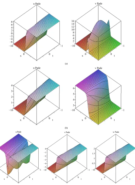
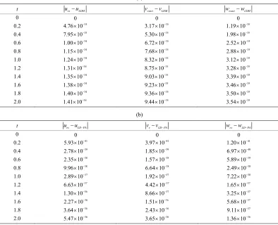
In this section we use Maple to calculate the [3/2] the Pade approximant of the infinite series solution (18), (23), and (28) which gives the rational fraction approximation to the solution, and Figures 4(a)-(c) show the results obtained by the Pade approximant (LD-PA) solution of systems (1), (3) and (5), and Figures 5(a)-(c) show comparison between the exact solution, LDM solution and the Pade approximant (LD-PA) solution of systems (1), (3) and (5) at, x = 5, −1 ≤t ≤ 1. Tables 1-3 show the absolute error

between the exact solution and the results obtained from the, LDM solution and the Pade approximant (LD-PA) solution of systems (1)-(3).

5. Conclusion

[image:5.595.129.471.81.455.2]

(6)

(a)

(b)

(c)

[image:6.595.107.493.73.711.2]

(7)

(a)

(b)

(c)

Figure 4. (a) The Pade approximant (LD-PA) solution of u(x, t) and v(x, t) of example 1, −10 ≤x≤ 10, −1 ≤t≤ 1; (b) The Pade

[image:7.595.78.525.77.692.2]

(8)

(a)

(b)

(c)

Figure 5. (a) The exact, (LDM)and the Pade approximant (LD-PA) solution of u(x, t) and v(x, t) of example 1, x = 5, −1 ≤t≤ 1; (b) The exact, (LDM)and the Pade approximant (LD-PA) solution of u(x, t) and v(x, t) of example 2, x = 5, −1 ≤t≤ 1; (c) The exact, (LDM)and the Pade approximant (LD-PA) solution of u(x, t), v(x, t) and w(x, t) of example 3, x = 5, −1 ≤t≤ 1.

which is capable of handling nonlinear system of partial differential equations. In this paper the (LDM) and Pade approximant has been successfully applied to find ap-

[image:8.595.64.536.77.640.2]

(9)

[image:9.595.102.495.101.222.2]

Table 1. The absolute error of u(x, t) and v(x, t) of example 1, x = 40.

t uexuLDM vexvLDM uexuLD PA– vexvLD PA–

0 0.2 0.4 0.6 0.8 1.0 1.2 1.4 1.6 1.8 2.0 0 2.56 × 10−69

6.38 × 10−69

1.20 × 10−68

2.06 × 10−68

3.32 × 10−68

5.22 × 10−68

8.05 × 10−68

1.22 × 10−67

1.85 × 10−67

2.79 × 10−67

0 1.02 × 10−69

2.55 × 10−69

4.83 × 10−69

8.24 × 10−69

1.33 × 10−67

2.08 × 10−67

3.21 × 10−67

4.90 × 10−67

7.42 × 10−67

1.11 × 10−66

0 4.16 × 10−75

3.79 × 10−73

6.24 × 10−72

5.14 × 10−71

2.90 × 10−70

1.29 × 10−69

4.81 × 10−69

1.54 × 10−68

4.33 × 10−68

1.05 × 10−67

0 1.66 × 10−74

1.51 × 10−72

2.49 × 10−71

2.05 × 10−70

1.16 × 10−69

5.16 × 10−69

1.92 × 10−68

6.19 × 10−68

1.73 × 10−67

[image:9.595.99.493.251.372.2]

4.22 × 10−67

Table 2. The absolute error of u(x, t) and v(x, t) of example 2, x = 40.

t uexuLDM vexvLDM uexuLD PA– vexvLD PA–

0 0.2 0.4 0.6 0.8 1.0 1.2 1.4 1.6 1.8 2.0 0 5.42 × 10−45

3.96 × 10−45

1.41 × 10−45

5.95 × 10−45

3.28 × 10−44

6.81 × 10−43

9.59 × 10−42

9.52 × 10−41

7.24 × 10−40

4.46 × 10−39

0 5.42 × 10−45

3.96 × 10−45

1.41 × 10−45

5.95 × 10−45

3.28 × 10−44

6.81 × 10−43

9.59 × 10−42

9.52 × 10−41

7.24 × 10−40

4.46 × 10−39

0 5.76 × 10−41

5.25 × 10−39

8.64 × 10−38

7.12 × 10−37

4.02 × 10−36

1.78 × 10−35

6.66 × 10−35

2.14 × 10−34

6.00 × 10−34

1.46 × 10−33

0 5.76 × 10−41

5.25 × 10−39

8.64 × 10−38

7.12 × 10−37

4.02 × 10−36

1.78 × 10−35

6.66 × 10−35

2.14 × 10−34

6.00 × 10−34

1.46 × 10−33

Table 3. (a) The absolute error of u(x, t), v(x, t) and w(x, t) of example 3, x = 40; (b) The absolute error of u(x, t), v(x, t) and w(x, t) of example 3, x = 40.

(a)

t uexuLDM vexactvLDM wexactwLDM

0 0.2 0.4 0.6 0.8 1.0 1.2 1.4 1.6 1.8 2.0 0 35 4.76 10_ 

35 7.95 10_ 

34 1.00 10_ 

34 1.15 10_ 

34 1.24 10_ 

34 1.31 10_ 

34 1.35 10

34



1.38 10

34



1.40 10

34



1.41 10

0 35 3.17 10_ 

35 5.30 10_ 

35 6.72 10_ 

35 7.68 10_ 

35 8.32 10_ 

35 8.75 10_ 

35 9.03 10

35



9.23 10

35



9.36 10

35



9.44 10

0 35 1.19 10_ 

35 1.98 10_ 

35 2.52 10_ 

35 2.88 10_ 

35 3.12 10_ 

35 3.28 10_ 

35 3.39 10

35



3.46 10

35



3.50 10

35



3.54 10

(b)

t uexuLD PA– vevLD PA– wexwLD PA–

0 0.2 0.4 0.6 0.8 1.0 1.2 1.4 1.6 1.8 2.0 0 41 5.93 10_ 

39 2.78 10_ 

38 2.35 10_ 

38 9.96 10_ 

37 2.89 10_ 

37 6.63 10_ 

36 1.30 10

36



2.27 10

36



3.64 10

36



5.47 10

0 41 3.97 10_ 

39 1.85 10_ 

38 1.57 10_ 

38 6.64 10_ 

37 1.92 10_ 

37 4.42 10_ 

37 8.66 10

36



1.51 10

36



2.43 10

36



3.65 10

0 41 1.20 10_ 

40 6.97 10_ 

39 5.89 10_ 

38 2.49 10_ 

38 7.22 10_ 

37 1.65 10_ 

37 3.25 10

37



5.68 10

37



9.11 10

36



[image:9.595.100.494.418.738.2]

(10)

KdV. It was noted that the scheme found the solutions without any discretization or restrictive assumption, and it was free from round-off errors and therefore reduced the numerical computations to a great extent.

REFERENCES

[1] S. A. Khuri, “A Laplace Decomposition Algorithm Ap- plied to Class of Nonlinear Differential Equations,” Jour- nal of Applied Mathematics, Vol. 1, No. 4, 2001, pp. 141- 155.

[2] H. Hosseinzadeh, H. Jafari and M. Roohani, “Application of Laplace Decomposition Method for Solving Klein- Gordon Equation,” World Applied Sciences Journal, Vol. 8, No. 7, 2010, pp. 809-813.

[3] M. Khan, M. Hussain, H. Jafari and Y. Khan, “Applica- tion of Laplace Decomposition Method to Solve Nonlin- ear Coupled Partial Differential Equations,” World Ap- plied Sciences Journal, Vol. 9, No. 1, 2010, pp. 13-19. [4] E. Yusufoglu (Aghadjanov), “Numerical Solution of Duff-

ing Equation by the Laplace Decomposition Algorithm,” Applied Mathematics and Computation, Vol. 177, No. 2, 2006, pp. 572-580. doi:10.1016/j.amc.2005.07.072 [5] T. Xu, J. Li and H.-Q. Zhang, “New Extension of the

Tanh-Function Method and Application to the Whitham- Broer-Kaup Shallow Water Model with Symbolic Com-

putation,” Physics Letters A, Vol. 369, No. 5-6, 2007, pp. 458-463. doi:10.1016/j.physleta.2007.05.047

[6] A. A. Solimana and M. A. Abdoub, “Numerical Solutions of Nonlinear Evolution Equations Using Variational It- eration Method,” Journal of Computational and Applied Mathematics, Vol. 207, No. 1, 2007, pp. 111-120.

doi:10.1016/j.cam.2006.07.016

[7] E. Fan, “Soliton Solutions for a Generalized Hirota-Sa- tsuma Coupled KdV Equation and a Coupled MKdV Equation,” Physics Letters A, Vol. 2852, No. 1-2, 2001, pp. 18-22. doi:10.1016/S0375-9601(01)00161-X

[8] H. Jafari and V. Daftardar-Gejji, “Solving Linear and Nonlinear Fractional Diffution and Wave Equations by Adomian Decomposition,” Applied Mathematics and Com- putation, Vol. 180, No. 2, 2006, pp. 488-497.

doi:10.1016/j.amc.2005.12.031

[9] F. Abdelwahid, “A Mathematical Model of Adomian Polynomials,” Applied Mathematics and Computation, Vol. 141, No. 2-3, 2003, pp. 447-453.

doi:10.1016/S0096-3003(02)00266-7