OSCILLATOR EQUATION BY DIFFERENCE EQUATIONS
JAN L. CIE ´SLI ´NSKI AND BOGUSŁAW RATKIEWICZReceived 29 October 2005; Accepted 10 January 2006
We discuss the discretizations of the second-order linear ordinary diffrential equations with constant coefficients. Special attention is given to the exact discretization because there exists a difference equation whose solutions exactly coincide with solutions of the corresponding differential equation evaluated at a discrete sequence of points. Such exact discretization can be found for an arbitrary lattice spacing.
Copyright © 2006 J. L. Cie´sli ´nski and B. Ratkiewicz. This is an open access article distrib-uted under the Creative Commons Attribution License, which permits unrestricted use, distribution, and reproduction in any medium, provided the original work is properly cited.
1. Introduction
The motivation for writing this paper is an observation that small and apparently not very important changes in the discretization of a differential equation lead to difference equa-tions with completely different properties. By the discretization we mean a simulation of the differential equation by a difference equation [5].
In this paper we consider the damped harmonic oscillator equation
¨
x+ 2γx˙+ω20x=0, (1.1)
wherex=x(t) and the dot means thet-derivative. This is a linear equation and its general solution is well known. Therefore discretization procedures are not so important (but sometimes are applied, see [3]). However, this example allows us to show and illustrate some more general ideas.
The most natural discretization, known as the Euler method (Appendix B, cf. [5,10]) consists in replacingxbyxn, ˙xby the difference ratio (xn+1−xn)/ε, ¨x by the difference ratio of difference ratios, that is,
¨ x−→1ε
x
n+2−xn+1
ε −xn+1ε−xn
=xn+2−2xn+1+xn
ε2 , (1.2)
Hindawi Publishing Corporation Advances in Difference Equations Volume 2006, Article ID 40171, Pages1–17
and so on. This possibility is not unique. We can replace, for instance,xbyxn+1, ˙xby (xn−
xn−1)/ε, or ¨x by (xn+1−2xn+xn−1)/ε2. Actually the last formula, due to its symmetry, seems to be more natural than (1.2) (and it works better indeed, seeSection 2).
In any case we demand that the continuum limit, that is,
xn=xtn, tn=εn,ε−→0, (1.3)
applied to any discretization of a differential equation yields this differential equation. The continuum limit consists in replacingxnbyx(tn)=x(t) and the neighboring values
are computed from the Taylor expansion of the functionx(t) att=tn:
xn+k=x
tn+kε=xtn+ ˙xtnkε+1 2x¨
tnk2ε2+···. (1.4)
Substituting these expansions into the difference equation and leaving only the leading term we should obtain the considered differential equation.
In this paper we compare various discretizations of the damped (and undamped) har-monic oscillator equation, including the exact discretization of the damped harhar-monic oscillator equation (1.1). By exact discretization we mean thatxn=x(tn) holds for anyε
and not only in the limit (1.3).
2. Simplest discretizations of the harmonic oscillator
Let us consider the following three discrete equations: xn+1−2xn+xn−1
ε2 +xn−1=0, (2.1)
xn+1−2xn+xn−1
ε2 +xn=0, (2.2)
xn+1−2xn+xn−1
ε2 +xn+1=0, (2.3)
whereεis a constant. The continuum limit (1.3) yields, in any of these cases, the harmonic oscillator equation
¨
x+x=0. (2.4)
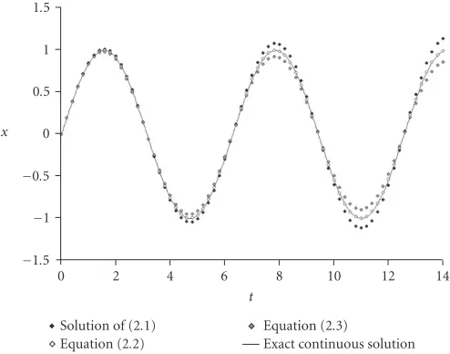
To fix our attention, in this paper we consider only the solutions corresponding to the initial conditionsx(0)=0, ˙x(0)=1. The initial data for the discretizations are chosen in the simplest form: we assume thatx0andx1belong to the graph of the exact continuous solution.
For smalltnand smallε, the discrete solutions of any of these equations approximate
1.5
1
0.5
0
−0.5
−1
−1.5
x
0 2 4 6 8 10 12 14
t
Solution of (2.1) Equation (2.2)
Equation (2.3)
Exact continuous solution
Figure 2.1. Simplest discretizations of the harmonic oscillator equation for smalltandε=0.02.
solution becomes increasingly different from the exact continuous solution even in the case (2.2) (cf. Figures2.2and2.3).
The natural question arises:how to find a discretization which is the best as far as global properties of solutions are concerned?
In this paper we will show how to find the “exact” discretization of the damped har-monic oscillator equation. In particular, we will present the discretization of (2.4) which is better than (2.2) and, in fact, seems to be the best possible. We begin, however, with a very simple example which illustrates the general idea of this paper quite well.
3. The exact discretization of the exponential growth equation
We consider the discretization of the equation ˙x=x. Its general solution reads
x(t)=x(0)et. (3.1)
The simplest discretization is given by xn+1−xn
ε =xn. (3.2)
This discrete equation can be solved immediately. Actually this is just the geometric se-quencexn+1=(1 +ε)xn. Therefore
xn=(1 +ε)nx0. (3.3)
To compare with the continuous case we write (1 +ε)nin the form
1.5
1
0.5
0
−0.5
−1
−1.5
x
3502 3504 3506 3508 3510 3512 3514 3516
t
Solution of (2.1) Equation (2.2)
Equation (2.3)
Exact continuous solution
Figure 2.2. Simplest discretizations of the harmonic oscillator equation for largetandε=0.02.
1.5
1
0.5
0
−0.5
−1
−1.5
x
9000 9005 9010 9015 9020
t
Exact discretization, (6.13) Equation (2.2)
Runge-Kutta scheme, (4.10) Exact continuous solution
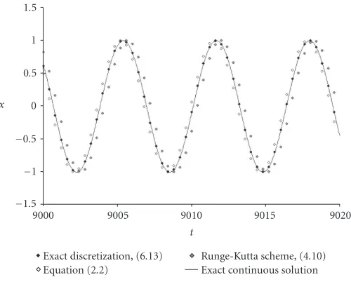
Figure 2.3. Good discretizations of the harmonic oscillator equation for largetandε=0.02.
wheretn:=εnandκ:=ε−1ln(1 +ε). Thus the solution (3.3) can be rewritten as
Therefore we see that forκ=1 the continuous solution (3.1), evaluated attn, that is,
xtn=x(0)etn, (3.6)
differs from the corresponding discrete solution (3.5). One can easily see that 0< κ <1. Only in the limitε→0 we haveκ→1.
Although the qualitative behavior of the “naive” simulation (3.2) is in good agreement with the smooth solution (exponential growth in both cases), but quantitatively the dis-crepancy is very large fort→ ∞because the exponents are different.
The discretization (3.2) can be easily improved. Indeed, replacing in the formula (3.3) 1 +εbyeεwe obtain that it coincides with the exact solution (3.6). This “exact discretiza-tion” is given by
xn+1−xn
eε−1 =xn, (3.7)
or, simply,xn+1=eεxn. Note thateε≈1 +ε(forε≈0) and this approximation yields (3.2).
4. Discretizations of the harmonic oscillator: exact solutions
The general solution of the harmonic oscillator equation (2.4) is well known:
x(t)=x(0) cost+ ˙x(0) sint. (4.1)
InSection 2we compared graphically this solution with the simplest discrete simulations: (2.1), (2.2), (2.3). Now we are going to present exact solutions of these discrete equations. Because the discrete case is usually less known than the continuous one, we recall shortly that the simplest approach consists in searching solutions in the formxn=Λn
(this is an analogue of the ansatzx(t)=exp(λt) made in the continuous case, for more details, seeAppendix A). As a result we get the characteristic equation forΛ.
We illustrate this approach on the example of (2.1) resulting from the Euler method. Substitutingxn=Λnwe get the following characteristic equation:
Λ2−2Λ+1 +ε2=0, (4.2)
with solutionsΛ1=1 +iε,Λ2=1−iε. The general solution of (2.1) reads
xn=c1Λn1+c2Λn2, (4.3)
and, expressingc1,c2by the initial conditionsx0,x1, we have
xn=x1(1 +iε)
n−(1−iε)n
2iε +x0
(1 +iε)(1−iε)n−(1−iε)(1 +iε)n
2iε . (4.4)
Denoting
1.5
1
0.5
0
−0.5
−1
−1.5
x
0 5 10 15 20
t
Exact discretization, (6.13) Equation (2.2)
Runge-Kutta scheme, (4.10) Exact continuous solution
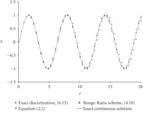
Figure 4.1. Good discretizations of the harmonic oscillator equation for smalltandε=0.4.
whereρ=√1 +ε2andα=arctanε, we obtain after elementary calculations
xn=ρn
x0cos(nα) +x1−x0 ε sin(nα)
. (4.6)
It is convenient to denoteρ=eκεand
tn=nε, κ:=21εln1 +ε2, ω:=arctanε ε, (4.7)
and then
xn=eκtn
x0cosωtn+x1−εx0sinωtn
. (4.8)
One can check thatκ >0 andω <1 for anyε >0. Forε→0 we haveκ→0,ω→1. There-fore the discrete solution (4.8) is characterized by the exponential growth of the envelope amplitude and a smaller frequency of oscillations than the corresponding continuous so-lution (4.1).
A similar situation is in the case (2.3), with only one (but very important) difference: instead of the growth we have the exponential decay. The formulas (4.7) and (4.8) need only one correction to be valid in this case. Namely,κhas to be changed to−κ.
The third case, (2.2), is characterized byρ=1, and, therefore, the amplitude of the oscillations is constant (this case will be discussed below in more detail).
Let us consider the following family of discrete equations (parameterized by real pa-rametersp,q):
xn+1−2xn+xn−1
ε2 +pxn−1+ (1−p−q)xn+qxn+1=0. (4.9) The continuum limit (1.3) applied to (4.9) yields the harmonic oscillator (2.4) for any p,q. The family (4.9) contains all three examples ofSection 2and (forp=q=1/4) the equation resulting from the Gauss-Legendre-Runge-Kutta method (seeAppendix B):
xn+1−2 4−ε2
4 +ε2
xn+xn−1=0. (4.10)
Substitutingxn=Λninto (4.9) we get the following characteristic equation:
1 +qε2Λ2−2 + (p+q−1)ε2Λ+1 +pε2=0. (4.11)
We formulate the following problem: find a discrete equation in the family (4.9) with the global behavior of solutions as much similar to the continuous case as possible.
At least two conditions seem to be very natural in order to get a “good” discretization of the harmonic oscillator: oscillatory character and a constant amplitude of the solutions (i.e.,ρ=1,κ=0). These conditions can be easily expressed in terms of roots (Λ1,Λ2) of the quadratic equation (4.11). First, the roots should be imaginary (i.e.,Δ<0), second, their modulus should be equal to 1, that is,Λ1=eiα,Λ2=e−iα. Therefore 1 +pε2=1 + qε2, that is,q=p. In the caseq=p, the discriminantΔof the quadratic equation (4.11) is given by
Δ= −4ε2+ε4(1−4p). (4.12)
There are two possiblities: ifp≥1/4, thenΔ<0 for anyε=0, and if p <1/4, thenΔ< 0 for sufficiently smallε, namelyε2<4(1−4p)−1. In any case, these requirements are not very restrictive and we obtained p-family of good discretizations of the harmonic oscilltor. IfΛ1=eiαandΛ2=e−iα, then the solution of (4.9) is given by
xn=x0costnω+x1−sinx0αcosαsintnω, (4.13)
whereω=α/ε, that is,
ω=1εarctan
ε
1 +ε2p−1/4 1 +p−1/2ε2
. (4.14)
Note that the formula (4.13) is invariant with respect to the transformationα→ −αwhich means that we can chooseΛ1as any of the two roots of (4.11).
Expanding (4.14) in the Maclaurin series with respect toε, we get
Therefore the best approximation of (2.4) from among the family (4.9) is characterized byp=1/12:
The standard numerical methods give similar results (in all cases presented in Appendix B, the discretization of the second derivative is the simplest one, the same as described in our introduction). The corresponding discrete equations do not simulate (2.4) better than the discretizations presented inSection 2.
5. Damped harmonic oscillator and its discretization
Let us consider the damped harmonic oscillator equation (1.1). Its general solution can be expressed by the rootsλ1,λ2of the characteristic equationλ2+ 2γλ+ω2
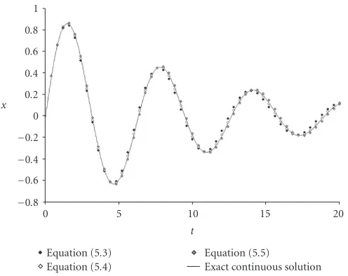
To obtain some simple discretization of (1.1), we should replace the first derivative and the second derivative by discrete analogues. The results ofSection 2suggest that the best way to discretize the second derivative is the symmetric one, like in (2.2). There are at least 3 possibilities for the discretization of the first derivative leading to the following simulations of the damped harmonic oscillator equation:
xn+1−2xn+xn−1
1 0.8 0.6 0.4 0.2 0
−0.2
−0.4
−0.6
−0.8
x
0 5 10 15 20
t
Equation (5.3) Equation (5.4)
Equation (5.5)
Exact continuous solution
Figure 5.1. Simplest discretizations of the weakly damped harmonic oscillator equation (ω0=1,γ=
0.1) for smalltandε=0.3.
6. The exact discretization of the damped harmonic oscillator equation
In order to find the exact discretization of (1.1) we consider the general linear discrete equation of second order:
xn+2=2Axn+1+Bxn. (6.1)
The general solution of (6.1) has the following closed form (cf.Appendix A):
xn=x0
Λ1Λn2−Λ2Λn1
+x1Λn1−Λn2
Λ1−Λ2 , (6.2)
whereΛ1,Λ2are roots of the characteristic equationΛ2−2AΛ−B=0, that is,
Λ1=A+ A2+B, Λ2=A− A2+B. (6.3)
The formula (6.2) is valid forΛ1=Λ2, which is equivalent toA2+B=0. If the eigenvalues coincide (Λ2=Λ1,B= −A2), we haveΛ1=Aand
xn=(1−n)Λ1x0n +nΛn1−1x1. (6.4)
Is it possible to identifyxngiven by (6.2) withx(tn)wherex(t)is given by (5.1)?
The crucial point consists in setting
The degenerate case,Λ1=Λ2(which is equivalent toλ1=λ2) can be considered analog-ically (cf.Appendix A). The formula (6.4) is obtained from (6.2) in the limitΛ2→Λ1. Therefore all formulas for the degenerate case can be derived simply by taking the limit λ2→λ1.
Thus we have a one-to-one correspondence between second-order differential equa-tions with constant coefficients and second-order discrete equations with constant co-efficients. This correspondence, referred to as the exact discretization, is induced by the relation (6.6) between the eigenvalues of the associated characteristic equations.
The damped harmonic oscillator (1.1) corresponds to the discrete equation (6.1) such that
In the case of the weakly damped harmonic oscillator (ω0> γ >0), the exact discretiza-tion is given by
A=e−εγcos(εω), B= −e−2εγ, (6.10)
whereω:=ω20−γ2. In other words, the exact discretization of (1.1) reads
xn+2−2e−εγcos(ωε)xn+1+e−2γεxn=0. (6.11)
The initial data are related as follows (see (6.8)):
1 0.8 0.6
0.4 0.2 0
−0.2
−0.4
−0.6
−0.8
x
0 5 10 15 20
t
Exact discretization, (6.11) Equation (5.4)
Runge-Kutta scheme, (B.8) Exact continuous solution
Figure 6.1. Good discretizations of the weakly damped harmonic oscillator equation (ω0=1,γ=0.1)
for smalltandε=0.2.
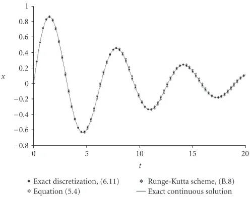
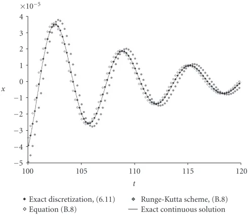
Figures6.1and6.2compare our exact discretization with two other good discretizations of the weakly damped harmonic oscillator. The exact discretization is really exact, that is, the discrete points belong to the graph of the exact continuous solution (for anyεand anyn). Similarly as in the undumped case, the fully symmetric simple discretization (5.4) is better than the equation resulting from the GLRK method.
The exact discretization of the harmonic oscillator equation ¨x+x=0 is a special case of (6.11) and is given by
xn+2−2(cosε)xn+1+xn=0. (6.13)
It is easy to verify that the formula (6.13) can be rewritten as xn+2−2xn+1+xn
2 sin(ε/2)2 +xn+1=0, (6.14)
which reminds the “symmetric” version of Euler’s discretization scheme (see (1.2) and (2.2)), but ε that appears in the discretization of the second derivative is replaced by 2 sin(ε/2). For smallεwe have 2 sin(ε/2)≈ε.
The solution of the initial value problem for (6.13) is given by
xn=x0cos(nε) +x1−sinx0εcosεsin(nε), (6.15)
(cf. (6.8)). Thus the discrete analogue ofx(0) is simplyx0, while the initial analogue of ˙
×10−5
4
3 2
1
0
−1
−2
−3
−4
−5
x
100 105 110 115 120
t
Exact discretization, (6.11) Equation (B.8)
Runge-Kutta scheme, (B.8) Exact continuous solution
Figure 6.2. Good discretizations of the weakly damped harmonic oscillator equation (ω0=1,γ=0.1)
for largetandε=0.2.
The comparison of the exact discretization (6.13) with three other discrete equations simulating the harmonic oscillator is done in Figures2.3and4.1. We point out that the considered simulations are very good indeed (althoughtinFigure 2.3is very large) but they cannot be better than the exact discretization. The discretization (4.16) is also excel-lent. The coefficient by−2xnin (4.16),
12−5ε2 12 +ε2 ≈1−
1 2!ε
2+ 1 4!ε
4+···, (6.16)
approximates cosεup to the 4th order. Actually, for the choice of parameteres made in Figures2.3 and4.1, the discretization (4.16) practically cannot be discerned from the exact one.
7. Conclusions
In this paper we have shown that for linear ordinary differential equations of second or-der with constant coefficients, there exists a discretization which simulates properly all features of the differential equation. The solutions of this discrete equation exactly coin-cide with the solutions of the corresponding differential equation evaluated at a discrete lattice. Such exact discretization can be found for an arbitrary lattice spacingε.
We point out that to achieve our goal, we had to assume an essential dependence of the discretization on the considered equation, in contrast to the standard numerical approach to ordinary differential equations where practically no assumptions are imposed on the considered system (i.e., universal methods, applicable for any equation, are considered) [7].
In the last years one can observe the development of the numerical methods which are applicable for some clases of equations (e.g., admitting Hamiltonian formulation) but are much more powerful (especially when global or qualitative aspects are considered) [6,13].
“Recent years have seen a shift in paradigm away from classical considerations which motivated the construction of numerical methods for ordinary differential equations. Traditionally the focus has been on the stability of difference schemes for dissipative sys-tems on compact time intervals. Modern research is instead shifting in emphasis towards the preservation of invariants and the reproduction of correct qualitative features” [9].
In our paper we have a kind of extremal situation: the method is applicable for a very narrow class of equations but as a result we obtain the discretization which seems to be surprisingly good. Linear ordinary differential equations with constant coefficients always admit the unique exact discretization. An interesting list of other ordinary differential equations possesing the exact discretization is presented in the book [1, Chapter 3].
Similar situation occurs for integrable nonlinear partial differential equations (soli-ton systems). It is believed (and proved for a very large class of equations) that inte-grable equations admit inteinte-grable discretizations which preserve the unique features of these equations (infinite number of conservation laws, solitons, transformations generat-ing explicit solutions, etc.) [2,4]. It would be interesting to compare standard integrable discretizations of KdV and modKdV equations (see, e.g., [14]) with discretizations con-structed in order to simulate in the best way one soliton solutions ([1]).
Appendices
A. Linear difference equations with constant coefficients
We recall a method of solving difference equations with constant coeficients. It consists in representing the equation in the form of a matrix equation of the first order. The general linear discrete equation of the second order,
xn+2=2Axn+1+Bxn, (A.1)
can be rewritten in the matrix form as follows:
yn+1=Myn, (A.2)
where
yn=
xn+1
xn
, M=
2A B
1 0
The general solution of (A.2) has, obviously, the following form:
yn=Mny0, (A.4)
and the solution of a difference equation is reduced to the purely algebraic problem of computing powers of a given matrix.
The same procedure can be applied for any linear difference equation with constant coefficients. If the difference equation is ofmth order, then to obtain (A.2), we define
yn:=xn+m,xn+m−1,...,xn+1,xn T
, (A.5)
where the superscriptTmeans the transposition.
The powerMncan be easily computed in the generic case in which the matrixMcan be diagonalized, that is, represented in the form
M=NDN−1, (A.6)
whereDis a diagonal matrix. Then, obviously,Mn=NDnN−1. The diagonalization is possible whenever the matrix M has exactly m linearly independent eigenvectors (in particular, if the characteristic equation (A.7) hasmpairwise different roots). Then the columns of the matrixNare just eigenvectors ofM, and the diagonal coefficients ofDare eigenvalues ofM.
where the columns ofNare the eigenvectors ofM, that is,
N=
and performing the multiplication we get (6.2).
it means thatM2=2AλM+B. In the case of the double root (B= −A2) one can easily prove by induction
Mn=(1−n)AnM+nAn−1. (A.11)
Substituting it to (A.2) we get immediately (6.4).
B. Numerical methods for ordinary differential equations
In this short note we give basic informations about some numerical methods for ordinary differential equations and we apply them to case of harmonic oscillator equation (2.4).
A system of linear ordinary differential equations (of any order) can always be rewrit-ten as a single matrix equation of the first order:
˙
y=Sy, (B.1)
where the unknown yis a vector andSis a given matrix (in generalt-dependent). Nu-merical methods are almost always (see [7]) constructed for a large class of ordinary differential equations (including nonlinear ones):
˙
y=f(t,y). (B.2)
We denote byyna numerical approximant to the exact solutiony(tn).
Euler’s method.
yk+1=yk+ε f
tk,yk. (B.3)
In this case the discretization of ¨x+x=0 is given by (2.1). Modified Euler’s methods.
yk+1=yk+ε f
tk+12ε,yk+12ε ftk,yk,
yk+1=yk+12εftk,yk+ftk+ε,yk+ε ftk,yk.
(B.4)
Both methods lead to the following discretization of ¨x+x=0: xn+1−2xn+xn−1
ε2 +xn+ 1 4ε
2x
n−1=0. (B.5)
The roots of the characteristic equation are imaginary and
Λ1=Λ2=1 +ε4
1-stage Gauss-Legendre-Runge-Kutta method.
The application of this numerical integration scheme yields the following discretization of the damped harmonic oscillator equation:
xn+1−2xn+xn−1
and the characteristic equation reads
Λ4−2Λ3+1 +9
This is an equation of the 4th order (with no real roots forε=0).
Acknowledgment
We are grateful to Prof. R. P. Agarwal for calling our attention to references [1,11,12] where the best (or exact) discretizations were introduced.
References
[1] R. P. Agarwal,Difference Equations and Inequalities, Monographs and Textbooks in Pure and Applied Mathematics, vol. 228, Marcel Dekker, New York, 2000.
[2] A. I. Bobenko, D. Matthes, and Yu. B. Suris, Discrete and smooth orthogonal systems: C∞ -approximation, International Mathematics Research Notices2003(2003), no. 45, 2415–2459. [3] M. M. de Souza,Discrete-to-continuum transitions and mathematical generalizations in the
clas-sical harmonic oscillator, preprint, 2003,hep-th/0305114v5.
[4] B. M. Herbst and M. J. Ablowitz,Numerically induced chaos in the nonlinear Schr¨odinger equa-tion, Physical Review Letters62(1989), no. 18, 2065–2068.
[6] A. Iserles and A. Zanna,Qualitative numerical analysis of ordinary differential equations, The Mathematics of Numerical Analysis (Park City, Utah, 1995) (J. Renegar, M. Shub, and S. Smale, eds.), Lectures in Applied Mathematics, vol. 32, American Mathematical Society, Rhode Island, 1996, pp. 421–442.
[7] J. D. Lambert,Numerical Methods for Ordinary Differential Systems, John Wiley & Sons, Chich-ester, 1991.
[8] S. Lang,Algebra, Addison-Wesley, Massachusetts, 1965.
[9] W. Oevel,Symplectic Runge-Kutta schemes, Symmetries and Integrability of Difference Equations (Canterbury, 1996) (P. A. Clarkson and F. W. Nijhoff, eds.), London Math. Soc. Lecture Note Ser., vol. 255, Cambridge University Press, Cambridge, 1999, pp. 299–310.
[10] D. Potter,Computational Physics, John Wiley & Sons, New York, 1973.
[11] R. B. Potts, Differential and difference equations, The American Mathematical Monthly 89 (1982), no. 6, 402–407.
[12] J. G. Reid,Linear System Fundamentals, Continuous and Discrete, Classic and Modern, McGraw-Hill, New York, 1983.
[13] A. S. Stuart,Numerical analysis of dynamical systems, Acta Numerica3(1994), 467–572. [14] Yu. B. Suris,The Problem of Integrable Discretization: Hamiltonian Approach, Progress in
Math-ematics, vol. 219, Birkh¨auser, Basel, 2003.
Jan L. Cie´sli ´nski: Instytut Fizyki Teoretycznej, Uniwersytet w Białymstoku, ul. Lipowa 41, 15-424 Białystok, Poland
E-mail address:[email protected]
Bogusław Ratkiewicz: Doctoral Studies, Wydział Fizyki, Uniwersytet Adama Mickiewicza, Pozna ´n, Poland