Deep Convolutional Neural Network Textual Features and Multiple Kernel Learning for Utterance level Multimodal Sentiment Analysis

Deep Convolutional Neural Network Textual Features and Multiple

Kernel Learning for Utterance-Level Multimodal Sentiment Analysis

Soujanya Poria

Temasek Laboratory,

Nanyang Technological

University, Singapore

[email protected]

Erik Cambria

School of Computer Engineering,

Nanyang Technological

University, Singapore

[email protected]

Alexander Gelbukh

Centro de Investigación en

Computación, Instituto

Politécnico Nacional, Mexico

www.gelbukh.com

Abstract

We present a novel way of extracting fea-tures from short texts, based on the acti-vation values of an inner layer of a deep convolutional neural network. We use the extracted features in multimodal senti-ment analysis of short video clips repre-senting one sentence each. We use the combined feature vectors of textual, vis-ual, and audio modalities to train a classi-fier based on multiple kernel learning, which is known to be good at heteroge-neous data. We obtain 14% performance improvement over the state of the art and present a parallelizable decision-level da-ta fusion method, which is much faster, though slightly less accurate.

1

Introduction

The advent of the Social Web has enabled any-one with a smartphany-one or computer to easily cre-ate and share their ideas, opinions and content with millions of other people around the world. Much of the content being posted and consumed online is video. With billions of phones, tablets and PCs shipping today with built-in cameras and a host of new video-equipped wearables like Google Glass on the horizon, the amount of vid-eo on the Internet will only continue to increase.

It has become increasingly difficult for re-searchers to keep up with this deluge of video content, let alone organize or make sense of it. Mining useful knowledge from video is a critical need that will grow exponentially, in pace with the global growth of content. This is particularly important in sentiment analysis (Cambria et al., 2013a; 2013b; 2014), as both service and product reviews are gradually shifting from unimodal to multimodal. We present a method for detecting

sentiment polarity in short video clips of a person uttering a sentence.

We do it using all three modalities: visual, such as facial expression, audio, such as pitch, and textual, the contents of the uttered sentence. While the visual and the audio modalities pro-vide additional epro-vidence that improves classifica-tion accuracy, we found the textual modality to have the greater impact on the result (Cambria and Hussain, 2015; Cambria et al., 2013c; Poria et al., 2015a; 2015b).

In this paper, we propose a novel way for fea-ture extraction from text. Given a training corpus with hand-annotated sentiment polarity labels, following Kim (2014), we train a deep convolu-tional neural network (CNN) on it. However, instead of using it as a classifier, as Kim did, we use the values from its hidden layer as features for a much more advanced classifier, which gives superior accuracy. Similar ideas have been sug-gested in the context of computer vision for deal-ing with images, but have not been applied in the context of NLP to textual data, and, specifically, for sentiment polarity classification.

2

Overview of the Method

In this paper, we present two different methods for dealing with multimodal data: feature-level fusion and decision-level fusion, each one having its advantages and disadvantages.

3

Textual Features

We used a CNN as a trainable feature extractor to extract features from the textual data. Utter-ances in the original dataset are in Spanish. While usually it is better to work directly with the source language (Wang et al., 2013), in this work we translated utterances into English using Google translator. Without the translation into English, 68.56% accuracy was obtained.

The choice of CNN for feature extraction is justified by the following considerations:

1. The convolution layers of CNN can be seen as a feature extractor, whose output is then fed into a rather simplistic classifier useful for training the network but not the best at actual classification. CNN forms local fea-tures for each word and combine them to produce a global feature vector for the whole text. However, the features that CNN builds internally can be extracted and used as input for another, more advanced classifier. This turns CNN, originally a supervised classifier, into a trainable feature extractor.

2. As a feature extractor, CNN is automatic and does not rely on handcrafted features. In par-ticular, it adapts well to the peculiarities of the specific dataset, in a supervised manner. 3. The features it gives are based on a hierarchy

of local features, reflecting well the context.

A drawback of CNN as a classifier is that it finds only a local optimum, since it uses the same backpropagation technique as MLP. How-ever, inspired by ideas introduced in the context of computer vision (Bluche et al., 2013), we, for the first time in the context of NLP, extract the features that CNN builds internally and feed them into a much more advanced classifier. In our experiments, this was SVM, or roughly its multi-kernel version MKL, which is good at finding the global optimum. Thus, the properties of CNN and SVM complement each other in such a way that their advantages are combined.

To form the input for the CNN feature extrac-tor, for each word in the text we built a 306-dimensional vector by concatenating two parts:

1. Word embeddings. We used a publicly

avail-able word2vec dictionary (Mikolov et al., 2013a; 2013b; 2013c), trained on a 100 mil-lion word corpus from Google News using the continuous bag of words architecture. This dictionary provides a 300-dimensional vector for each word. For words not found in this dictionary, we used random vectors.

2. Part of speech. We used 6 basic parts of

speech (noun, verb, adjective, adverb, prepo-sition, conjunction) encoded as a 6-dimensional binary vector. We used Stanford Tagger as a part of speech tagger.

For each input text, the input vectors for the CNN were a concatenation of three parts:

1. Left padding. Two dummy “words” with zero vectors were added at the beginning of each text, in order to provide space for con-volution, since at the convolution layers we used the kernel size of at most 3.

2. Text. All 306-dimensional vectors corre-sponding to each word were concatenated, preserving the word order.

3. Right padding. Again, at least 2 dummy “words” with zero vectors were added after each sentence to provide space for convolu-tion. To form vectors for all texts in the cor-pus of the same dimensionality, they were al-so padded at the right with the necessary amount of additional dummy “words.”

In our experiments, all texts were very short, consisting of one sentence, the longest one being of 65 words. Thus all input vectors were of di-mension 306  (2 + 65 + 2) = 21,114.

The CNN we used consisted of 7 layers:

1. Input layer, of 21,114 neurons.

2. Convolution layer, with a kernel size of 3 and 50 feature maps. The output of this layer was computed with a non-linear function; we used the hyperbolic tangent.

3. Max-pool layer with max-pool size of 2. 4. Convolution layer: kernel size of 2, 100

fea-ture maps, also using the hyperbolic tangent. 5. Max-pool layer with max-pool size of 2. 6. Fully connected layer of 500 neutrons,

whose values were later used as the extracted features. For regularization, we employed dropout on the penultimate layer with a con-straint on L2-norms of the weight vectors. 7. Output softmax layer of 2 neurons, by the

number of training labels—the sentiment po-larity values: positive or negative. This layer was used only for training the CNN.

layer of the CNN only for training, but for actual decision-making, we replaced it with much more sophisticated classifiers, namely, with SVM or MKL. Using only CNN as a classifier, 75.50% was obtained which is in fact lower than the re-sult (79.77%) obtained when CNN was used to extract trainable features for the SVM classifier.

We also tried other word vectors having dif-ferent dimensions, e.g., Glove word vectors and Collobart’s word vectors. However, the best ac-curacy was obtained using Google word2vec.

4

Visual Features

We split each clip into frames (still images). From each frame, we extracted 68 facial charac-teristic points (FCPs), such as the position of the left corner of the left eye, etc., using the facial recognition library CLM-Z (Baltrušaitis et al., 2012). For each pair of FCPs, we calculated the distance. Thus, we characterized each facial ex-pression by 68  67 / 2 = 2,278 distances. In ad-dition, for each frame we extracted 6 face posi-tion coordinates (3D-dimensional displacement and angular displacement of face and head) using the GAVAM software. This gave 2,278 + 6 = 2,284 values per frame.

For each of these values, we calculated its mean value and standard deviation over all frames of the clip; 4568 features in total.

5

Audio Features

We used the openSMILE software (Eyben et al., 2010) to extract audio features related to the pitch and voice intensity. This software extracts the so-called low-level descriptors, such as Mel frequency cepstral coefficients, spectral centroid, spectral flux, beat histogram, beat sum, strongest beat, pause duration, pitch, voice quality,

percep-tual linear predictive coefficients, etc., and their statistical functions, such as amplitude mean, arithmetic mean, root quadratic mean, standard deviation, flatness, skewness, kurtosis, quartiles, inter-quartile ranges, linear regression slope, etc. This gave us 6373 audio features in total.

6

Feature-Level Fusion

Feature-level fusion consisted in concatenation of the feature vectors obtained for each of the three modalities. The resulted vectors and along with the sentiment polarity labels from the train-ing set, were used to train a classifier with a mul-tiple kernel learning (MKL) algorithm; we used the SPF-GMKL implementation (Jain et al., 2012) designed to deal with heterogeneous data. Clearly, feature vectors resulted from concatenat-ing so different data sources are heterogeneous.

The parameters of the classifier were found by cross validation. We chose a configuration with 8 kernels: 5 RBF with gamma from 0.01 to 0.05 and 3 polynomial with powers 2, 3, 4. We also tried Simple-MKL; it gave slightly lower results.

7

Feature Selection

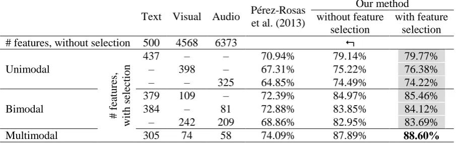
We significantly reduced the number of features using feature selection. We used two different feature selectors: one based on the cyclic correla-tion-based feature subset selection (CFS) and another based on principal component analysis (PCA) with top K features, where K was experi-mentally selected and varied for different exper-iment. For example, in case of audio, visual and textual fusion, K was set to 300.

The union of the features selected by the two methods was used. For each unimodal, each bi-modal, and the multimodal experiment, separate feature extraction was performed. The number of Text Visual Audio Pérez-Rosas

et al. (2013)

Our method without feature

selection

with feature selection # features, without selection 500 4568 6373 

Unimodal

# f

ea

tu

res

,

w

it

h s

el

ec

ti

on

437 – – 70.94% 79.14% 79.77%

– 398 – 67.31% 75.22% 76.38%

– – 325 64.85% 74.49% 74.22%

Bimodal

379 109 – 72.39% 84.97% 85.46% 384 – 81 72.88% 83.85% 84.12% – 242 209 68.86% 82.95% 83.69%

Multimodal 305 74 58 74.09% 87.89% 88.60%

selected features for each experiment is given in Table 1. In all cases except for the unimodal ex-periment with audio modality, feature selection slightly improved the results, in addition to the improvement in processing time. In the only case where feature selection slightly deteriorated the result, the difference was rather small.

8

Unimodal Classification and

Decision-Level Fusion

For unimodal experiments and for decision-level fusion, we used one classifier per each modality; specifically, we used SVM. For each modality, in this way we obtained the probabilities of the bels. In unimodal experiments, we chose the la-bel with the greater probability.

For decision-level fusion, we added these probabilities with weights, which were chosen experimentally, and, again, used the most proba-ble label. The weights we used for decision-level fusion were chosen using detailed search with an intuition that best performing unimodal classifier has higher importance in the fusion. We do not claim that these weights are optimal. They are indeed sub-optimal and hence encourage the scope of future research.

Knowing a specific decision for the text mo-dality allowed us to use evidence from a separate classifier; we used the one based on the Sentic Patterns (SP) (Poria et al., 2014a). It structures natural language clauses into a sentiment hierar-chy used to infer the overall polarity label (posi-tive vs. nega(posi-tive) for the input sentence. E.g., a sentence “The car is very old but it is rather not expensive”, is positive, expressing a favorable sentiment of the speaker, who recommends pur-chasing the product. However, “The car is very old though it is rather not expensive” is negative, expressing reluctance of the speaker to purchase the car. Despite the latter contains exactly the same concepts as the former, the polarity is op-posite because of the adversative dependency.

On benchmark datasets, SP perform better than state of the art sentiment classifiers, which outperforms the textual classifier described in Section 3. Since SP are a superior classifier, we used it as a bias to modify the weight of the tex-tual modality. However, SP do not report a prob-ability, but only a binary decision, so we only used them to tweak the weights in the probability mix: when the text-based unimodal classifier agreed with SP, we increased the weight of the text modality. Another benefit of the decision-level fusion is its speed, since fewer features are

used for each classifier and since SVM, used as a unimodal classifier, is faster than MKL. In addi-tion, separate classifiers can be run in parallel.

9

Experimental Results

We report results for tenfold cross-validation.

9.1 Dataset

We experimented on the dataset described by Morency et al. (2011). The dataset consists of 498 short video fragments where a person utters one sentence. The items are manually tagged for sentiment polarity, which can be positive, nega-tive, or neutral. We discarded the neutral items from the dataset, which gave us a dataset of 447 clips tagged as positive or negative.

The video in the dataset is present in MP4 format with the resolution of 360  480, to which the developers converted all videos originally collected in different formats with different reso-lution. The duration of the clips is about 5 sec-onds on average. About 80% of the clips present female speakers. The developers provided tran-scription of the text of the sentences, which we used in our textual modality processing.

9.2 Results for Each Modality Separately

As a baseline, we used classifiers trained on fea-tures extracted from each modality separately. The results are shown in Table 1, unimodal sec-tion. The number of features after feature selec-tion is indicate for the modality used.

The table shows that the best results were ob-tained for textual modality; the visual modality performed worse, and the audio was least useful. However, even the worst of our results is much better than the state-of-the-art (Pérez-Rosas et al., 2013). In each modality separately, our re-sults outperform the state of the art by about 9%, which is about 30% reduction in error rate.

9.3 Results with Feature-level Fusion

As a yet another baseline, we tried feature-level fusion of only two modalities.

The results are shown in Table 1, bimodal sec-tion. Again, the number of features after feature selection is indicated for the two modalities used. As expected, missing the audio features was the least important, missing the video features was more significant, and missing the text features was most painful for the accuracy.

art. Finally, the best result, shown in the multi-modal section of Table 1, was obtained when all three modalities were fused. This result outper-forms the corresponding result of the state of the art by 14%, which gives 56% of error reduction.

9.4 Results with Decision-level Fusion

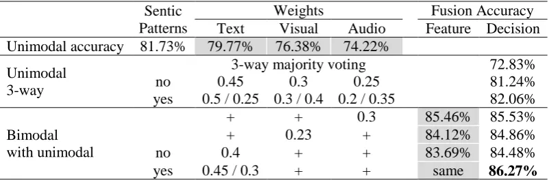
The results for decision-level fusion are shown in Table 2, last column. The shaded cells are shared with Table 1. In the second section, three classi-fiers were fused at the decision level. In the third section, two modalities indicated with the plus sign were fused at the feature level (giving the accuracy indicated in the penultimate column) and then this classifier was fused at the decision level with the third modality. The weights corre-spond to the share of each modality. In the last section, the weight for the unimodal classifier is shown, and the weight for the bimodal classifier was its complement to 1.

For the experiments that involved tweaking of the weights with the SP oracle, pairs of weights are shown: the weight used when the text mo-dality results corresponded (left) with the SP prediction and the weight used when they did not (right). The accuracy with at least partial level fusion was better than that for no feature-level fusion at all (3-way). As in the bimodal sec-tion of Table 1, excluding audio from feature-level fusion was least problematic and excluding text was most problematic.

In all cases, decision-level fusion did not sig-nificantly improve the accuracy of the best sum-mand. However, separating text-based classifier permitted us to use the Sentic Patterns tweak, which cannot be used if the text-only results are not known. With this tweak, the best result was obtained. Even with this improvement, the accu-racy of decision-level fusion was slightly lower than that of feature-level fusion; in exchange for much about twice better processing speed.

A baseline decision level evaluation strategy was taken which allowed us to take majority vot-ing among the predicted class labels by unimodal classifiers. Based on this strategy the final class label was chosen by the maximum of the three unimodal models’ votes. For the multimodal fu-sion using this baseline method only 72.83% ac-curacy was obtained. As expected the proposed feature and decision level fusion outperformed this baseline method by a large margin.

10

Conclusion

We have presented a novel method for determin-ing sentiment polarity in video clips of people speaking. We combine evidence from the words they utter, the facial expression, and the speech sound. The main novelty of this paper consists in using deep CNN to extract features from text and in using MKL to classify the multimodal hetero-geneous fused feature vectors.

We also presented a faster variant of our method, based on decision-level fusion. In case of the decision level fusion experiment, the cou-pling of Sentic Patterns to determine the weight of textual modality has enriched the performance of multimodal sentiment analysis framework considerably. However, the parameter selection for decision level fusion produced suboptimal results. A systematic mathematical approach for decision level fusion is an important future work. Our future work will focus on extracting more relevant features from the visual modality. We will employ deep 3D convolutional neural net-works on this modality for feature extraction. We will use a feature selection method to obtain key features; this will ensure the scalability as well as stability of the framework. We will continue our study of reasoning over text (Jimenez et al., 2015; Pakray et al., 2011; Sidorov et al., 2014; Sidorov, 2014) and in particular of concept-based sentiment analysis (Poria et al., 2014b). Sentic

Patterns

Weights Fusion Accuracy Text Visual Audio Feature Decision Unimodal accuracy 81.73% 79.77% 76.38% 74.22%

Unimodal 3-way

3-way majority voting 72.83%

no 0.45 0.3 0.25 81.24%

yes 0.5 / 0.25 0.3 / 0.4 0.2 / 0.35 82.06%

Bimodal with unimodal

+ + 0.3 85.46% 85.53%

+ 0.23 + 84.12% 84.86%

no 0.4 + + 83.69% 84.48%

yes 0.45 / 0.3 + + same 86.27%

References

1. Tadas Baltrušaitis, Peter Robinson, and Louis-Philippe Morency. 2012. 3D constrained local model for rigid and non-rigid facial tracking. In IEEE Conference on Computer Vision and Pat-tern Recognition (CVPR), pp. 2610–2617.

2. Théodore Bluche, Hermann Ney, and Christo-pher Kermorvant. 2013. Feature extraction with convolutional neural networks for handwritten word recognition. In 12th International Confer-ence on Document Analysis and Recognition (ICDAR), pp. 285–289.

3. Erik Cambria and Amir Hussain. 2015. Sentic Computing: A Common-Sense-Based Frame-work for Concept-Level Sentiment Analysis. Springer, Cham, Switzerland.

4. Erik Cambria, Björn Schuller, Bing Liu, Haixun Wang, and Catherine Havasi. 2013a. Knowle-dge-based approaches to concept-level sentiment analysis. IEEE Intelligent Systems 28(2):12–14.

5. Erik Cambria, Björn Schuller, Bing Liu, Haixun Wang, and Catherine Havasi. 2013b. Statistical approaches to concept-level sentiment analysis. IEEE Intelligent Systems 28(3):6–9.

6. Erik Cambria, Haixun Wang, and Bebo White. 2014. Guest editorial: Big social data analysis. Knowledge-Based Systems 69:1–2.

7. Erik Cambria, Newton Howard, Jane Hsu, and Amir Hussain. 2013c. Sentic blending: Scalable multimodal fusion for the continuous interpreta-tion of semantics and sentics. In: IEEE SSCI, pp. 108–117, Singapore.

8. Florian Eyben, Martin Wöllmer, and Björn Schuller. 2010. OpenSMILE: The Munich versa-tile and fast open-source audio feature extractor. In Proceedings of the International Conference on Multimedia, pp. 1459–1462.

9. Ashesh Jain, Swaminathan V. N. Vishwanathan, and Manik Varma. 2012. SPF-GMKL: General-ized multiple kernel learning with a million ker-nels. In Proceedings of the 18th ACM SIGKDD International Conference on Knowledge Discov-ery and Data Mining, pp. 750–758.

10. Sergio Jimenez, Fabio A. Gonzalez, and Alexan-der Gelbukh. 2015. Soft Cardinality in Semantic Text Processing: Experience of the SemEval In-ternational Competitions. Polibits 51:63–72.

11. Yoon Kim. 2014. Convolutional Neural Net-works for Sentence Classification. In EMNLP, pp. 1746–1751.

12. Tomas Mikolov, Kai Chen, Greg Corrado, and Jeffrey Dean. 2013a. Efficient estimation of word representations in vector space. In Intern. Conference on Learning Representations (ICLR).

13. Tomas Mikolov, Ilya Sutskever, Kai Chen, Greg Corrado, and Jeffrey Dean. 2013b. Distributed representations of words and phrases and their compositionality. In NIPS.

14. Tomas Mikolov, Wen-tau Yih, and Geoffrey Zweig. 2013c. Linguistic regularities in continu-ous space word representations. In NAACL-HLT.

15. Louis-Philippe Morency, Rada Mihalcea, and Payal Doshi. 2011. Towards multimodal senti-ment analysis: Harvesting opinions from the web. In 13th International Conference on Multi-modal Interfaces, pp. 169–176.

16. Verónica Pérez-Rosas, Rada Mihalcea, and Lou-is-Philippe Morency. 2013. Utterance-Level Multimodal Sentiment Analysis. In ACL, pp. 973–982.

17. Partha Pakray, Snehasis Neogi, Pinaki Bhaskar, Soujanya Poria, Sivaji Bandyopadhyay, and Al-exander Gelbukh. 2011. A textual entailment system using anaphora resolution. In: System Re-port. Text Analysis Conference, Recognizing Textual Entailment Track. Notebook.

18. Soujanya Poria, Erik Cambria, Gregoire Winter-stein, and Guang-Bin Huang. 2014a. Sentic pat-terns: Dependency-based rules for concept-level sentiment analysis. Knowledge-Based Systems 69:45–63.

19. Soujanya Poria, Erik Cambria, Amir Hussain, and Guang-Bin Huang. 2015a. Towards an intel-ligent framework for multimodal affective data analysis. Neural Networks 63:104–116.

20. Soujanya Poria, Erik Cambria, Newton Howard, Guang-Bin Huang, and Amir Hussain. 2015b. Fusing audio, visual and textual clues for senti-ment analysis from multimodal content. Neuro-computing, DOI: 10.1016/j.neucom.2015.01.095

21. Soujanya Poria, Alexander Gelbukh, Erik Cam-bria, Amir Hussain, and Guang-Bin Huang. 2014b. EmoSenticSpace: A novel framework for affective common-sense reasoning. Knowledge-Based Systems 69:108–123.

22. Grigori Sidorov, Alexander Gelbukh, Helena Gómez-Adorno, and David Pinto. 2014. Soft Similarity and Soft Cosine Measure: Similarity of Features in Vector Space Model. Com-putación y Sistemas 18(3):491–504.

23. Grigori Sidorov. 2014. Should Syntactic N-grams Contain Names of Syntactic Relations? In-ternational Journal of Computational Linguistics and Applications 5(2):23–46.