R E S E A R C H
Open Access
Improvement on the vanishing component
analysis by grouping strategy
Xiaofeng Zhang
1,2Abstract
Vanishing component analysis (VCA) method, as an important method integrating commutative algebra with machine learning, utilizes the polynomial of vanishing component to extract the features of manifold, and solves the classification problem in ideal space dual to kernel space. But there are two problems existing in the VCA method: first, it is difficult to set a threshold of its classification decision function. Second, it is hard to handle with the over-scaled training set and oversized dimension of eigenvector. To address these two problems, this paper improved the VCA method and presented a grouped VCA (GVCA) method by grouping strategy. The classification decision function did not use a predetermined threshold; instead, it solved the values of all polynomials of vanishing component and sorted them, and then used majority voting approach to determine their classes. After that, a strategy of grouping training set was proposed to segment training sets into multiple non-intersecting subsets, which polynomials of vanishing component were later acquired through a VCA method, respectively, and finally combined into an integral set of vanishing component polynomial. What is more important is that it uses the bagging theory in ensemble learning to successfully expound and prove the correctness of the strategy of grouping training sets. It also compares the time complexity for training algorithm with and without grouping training sets, thus demonstrating the effectiveness of the grouping strategy. A series of experiments showed that the GVCA method proposed in the paper has a perfect classification performance with a rapid rate of convergence compared to other statistical learning methods.
Keywords:VCA, Vanishing ideal, Ideal
1 Introduction
Commutative algebra is a discipline of algebra mainly studying commutative ring [1]. It takes the algebraic number theory and algebraic geometry as its study back-ground. In a classic sense, the research object of com-mutative algebra is the zero point of a polynomial equation set, which correlates with not only the number theory (such as Diophantine equation [2]) but also the manifold pattern (such as the hypersurface defined by polynomial) [3]. While, in a modern sense, the research object of commutative algebra is the topological space with rich structure (structure sheaf ) that could be pro-vided by a spectrum of a commutative ring. Commuta-tive algebra integrated with a manifold pattern has been widely applied in machine learning in recent years, as it
can solve some common machine learning problems, such as classification and clustering, from a perspective of a manifold pattern. Vanishing component analysis (VCA) [4] is a method of solving classification problem by applying the theory of commutative algebraic that has emerged in recent years. Therein, the vanishing compo-nent refers to a generator (i.e., Grobner basis [5]) for vanishing ideal of polynomial ring space of fitting a manifold pattern, which is in form of a group of polyno-mials employing feature as their variable. Once acquiring the vanishing component, the natural feature of a data manifold pattern can be captured.
The VCA method uses an ideal space dual to kernel space [6], thus becoming a dual algorithm of a kernel method. However, the VCA method has two problems: (1) A set of polynomials obtained through the VCA method, i.e., vanishing component, should be judged whether it is zero or not, when a test sample is substituted into a classification decision function. But in Correspondence:[email protected]
1Department of Computer Science and Engineering of Southeast University,
Nanjing, China
2
Jiangsu Administration Institute, Nanjing, China
the case of noise, it is difficult to ensure it is strictly zero. Even if a threshold is used, it is impossible to set its value. (2) The VCA method faces a similar difficulty with kernel method, that is, restriction on the scale of train-ing set [7]. This is because, in training algorithm, the number of training samples will influence the number of vanishing component polynomials, the number of mo-nomials contained in vanishing component polymo-nomials, the order of polynomial, etc. [4], thereby largely increasing the amount of calculation. On the other hand, an over-sized eigenvector dimension will also lead to an overover-sized dimension of singular value decomposition (SVD) matrix used in the VCA method, and finally make it harder to solve.
To solve the above two problems of the VCA method, this paper made a theoretical analysis and experimental research to improve the VCA method and presented a grouped VCA (abbreviated as GVCA) method. The GVCA method modified the classification decision func-tion in the VCA method. It did not preset a threshold; instead, it solved the values of all polynomials of vanish-ing component and sorted them, and then used the ma-jority voting approach to determine their classes. After that, a strategy of grouping training set was proposed on the basis of deduction of ensemble learning theory. In this strategy, the training sets were horizontally or verti-cally segmented into multiple non-intersecting subsets, which polynomials of vanishing components were later acquired through the VCA method, respectively, and fi-nally combined into an integral set of vanishing compo-nent polynomials. By experiment, it is verified that the GVCA method has a perfect classification performance with a rapid rate of convergence.
The main contributions of this paper include that (1) it proposed a classification decision function easier to operate, (2) it put forward a strategy of grouping train-ing sets and utilized the Baggtrain-ing theory in ensemble learning to successfully expound and prove the correct-ness of the strategy of grouping training sets, and (3) it deduced the time complexity for training algorithm after grouping, thus demonstrating the effectiveness of such strategy.
The paper is arranged as below: Section 2 introduces the efforts related to commutative algebra, the VCA method, and ensemble learning. Section 3 firstly pro-vides the theoretical basis of commutative algebra, then gives the VCA method and analyzes the problems caused by the threshold of its decision function being hard to set, and over-scaled training sets and oversized dimension of eigenvector. Finally, based on the analysis of problems resulted from setting threshold of a deci-sion function in the VCA method and proposed an improved decision function on the basis of sorted value of vanishing component polynomial, the experiment
showed that such improved decision function was more operational. Furthermore, based on the analysis of problems brought by the over-scaled training set and the oversized dimension of eigenvector, this section raised a strategy which horizontally and vertically grouped the training sets, made analysis on vanishing components respectively, and classified the union of vanishing component in each group. Then, the ensem-ble learning theory was utilized to verify the correct-ness and effectivecorrect-ness of this strategy. By improving these two aspects, a GVCA method was formed. After-wards, In Section 4, four experiments were conducted with simulation dataset and UCI dataset, which indi-cates that this method has a perfect classification per-formance with a rapid rate of convergence. At last, Section 5 presents a conclusion and forecast of the future work.
2 Related work 2.1 Commutative algebra
From the late eighteenth to the mid-nineteenth century, Gauss and Kummer et al. studied the nature of rational integer and the rational integer solution of equation and considered the Elementary Number Theory prob-lems in the quadratic field, cyclotomic field, and their algebraic integer ring [8, 9]. Through abstraction and systematization implemented by Dedekind and Hilbert et al. [10,11], a new discipline generated to study alge-braic number field and its algealge-braic integer ring, called Algebraic Number Theory [12]. In 1882, the concepts of the Ideal and the Prime Ideal proposed by Dedekind [13] laid a foundation for one-dimensional commuta-tive algebra [14]. At the time later than the number theory, geometry also experienced an algebraization process, and thus the multidimensional commutative algebra started to form its shape [15]. The Ideal Theory [16] proposed by Hilbert et al. at the end of nineteenth century and Noether in the 1920s to the 1930s, and the Valuation Theory [17], the Local Ring Theory [18], and the Dimension Theory [19] established by Krull have furnished classical geometry with brand new algebraic tools and enabled commutative algebra to be an inde-pendent discipline.
2.2 VCA method
is a result of commutative algebra combined with ma-chine learning, while the key is to apply commutative algebra in solving the generator for vanishing ideal of fitting manifold pattern. As data often contains noises, it is difficult to acquire an analytical solution, so numerical methods are needed to solve an ap-proximate vanishing ideal. The VCA method-related research involves as follows: Buchberger and Möller et al. firstly proposed an algorithm to figure out the vanishing ideal of finite point set, called Buchberger-Möller algorithm [20], which can be regarded as the Euclidean algorithm that solves the maximum com-mon divisor of single variable and the generalization of Gaussian elimination method in a linear system. The obtained Grobner basis has stable values when the coordinate system is measurable [21]. Corless et al. raised a singular value decomposition (SVD) [22] ap-proach for polynomial system and used it to solve the maximum common divisor problem [23], while SVD is the main step for solving the approximate vanishing ideal. Stetter developed the theory proposed by Corless et al. and presented a more general numerical method [24]. Heldt et al. utilized SVD and stable numerical method [25] to solve the approximate vanishing ideal, and these vanishing component polynomials almost composed a border basis [21]. Heldt et al. also worked out the Cohen-Macaulay basis of vanishing ideal [26]. Sauer et al. made use of a strategy of independent co-ordinate and increased degree of polynomial to calcu-late the approximate vanishing ideal, thereby acquiring an approximate solution of Buchberger-Möller algo-rithm [27]. Kiral et al. raised two dualities, namely, the duality between kernel and ideal and the duality be-tween ideal and manifold pattern. Then, these two dualities can be used to design two algorithms: ideal principal component analysis (IPCA) and approximate vanishing ideal component analysis (AVICA), in order to learn the generation features and discriminant fea-tures of manifold pattern [28]. Both algorithms can be considered as an extension of kernel primary compo-nent analysis (Kernel PCA) algorithm [29]. To sum up, commutative algebra provides an approach to solve the approximate vanishing ideal, and the VCA method uses an ideal space dual to kernel space, thus becoming a dual algorithm of kernel method. This has offered a new idea for solving machine learning problem in ker-nel space and is of great value in studying kerker-nel method and machine learning.
2.3 Ensemble learning
Ensemble learning refers to a kind of machine learn-ing method which uses a lot of learnlearn-ing devices to study and then integrates each learning outcome under some certain rules, so that the model’s stability
and prediction ability can be enhanced. Kleinberg proposed a general stochastic discrimination (SD) method to segment multidimensional space by sto-chastic process [30]. The SD method is capable to en-hance the performance of weak classifier. Based on this, Ho raised a random subspace method (RSM) and constructed a forest with the idea of RSM and the decision tree [31]. Hansen and Salamon proved that introducing ensemble learning into artificial neural network can improve the properties [32]. On the basis of random decision forest (RDF), Breiman employed the Bagging (i.e., bootstrap aggregation) technology, made a theoretical analysis, and provided an error upper-bound [33]. Bagging attempted to achieve similar learning module in small sample set, and then averaged the predicted values. This method uses different learning modules in different datasets to reduce the variance. Schapire put forward a boost-ing method [34], an iterative technique regulating the weight of observed value based on the last classifica-tion. If an observed value has been wrongly classified, it will increase the weight of observed values, and vice versa. Generally, boosting can decrease offset error to build a powerful prediction model. But some-times, it can also over-fit the training data. Freund and Schapire proposed an Adaboost method [35]. Cho and Kim integrated the results of multiple neural networks that used fuzzy logic, and the experiment showed this method improved the precision of classification [36]. The stacking approach raised by Wolpert is suitable to integrate different types of models and helps to bring offset error and variance down [37].
3 Methodology 3.1 Theoretical basis
Definition 1 (Left Ideal). The nonempty subset I⊆R in ringRis called the left ideal inR, ifIsatisfies the follow-ing two conditions [13]:
(1) The addition operation ofIin ringRconstitutes a subgroup of additive group of ringR.
(2)RI⊆R, i.e., for∀a∈Randb∈R, it satisfies
ab∈R.
Definition 2 (Right Ideal). The nonempty subset I⊆R in ring R is called the right ideal in R, if Isatisfies the following two conditions [13]:
(1) The addition operation ofIin ringRconstitutes a subgroup of additive group of ringR.
(2)IR⊆R, i.e., for∀a∈Randb∈R, it satisfies
Definition 3 (Ideal). IfIis both left ideal and right ideal, thenIis called a bi-ideal, abbreviated as Ideal [13].
Definition 4 (Vanishing Ideal). Givenkis a domain, and f1,f2,…,fmis a polynomial in the ringk[x1,x2,…,xn], then,
the set V can be defined as below:
V(f1,f2,…,fm) = {(u1,u2,…,un)∈kn:fi(u1,u2,…,un) = 0}.
In which, i= 1, 2,…, m. The set V(f1,f2,…,fm) is called
an affine variety of the polynomialf1,f2,…,fm. Then the
set I(V) = {f∈k[x1,x2,…,xn] :f(u1,u2,…un) = 0,∀u∈V} is
an ideal of the ring k[x1,x2,…,xn], called the vanishing
ideal of V [37].
Definition 5 (Grobner basis). Fix a monomial, if it satisfies the following formula, then a finitely gener-ated G=g1, …, gk will be the Grobner basis of ideal I [5].
LT gð Þ;1 …;LT gk
¼hLT Ið Þi ð1Þ
in which, LT(f ) represents the leading type of non-zero polynomial f. The coefficient of leading type is called a leading coefficient, denoted as LC(f ), and the corre-sponding term is called a leading term, denoted as LM(f ).
Example 1. For a non-zero polynomial f(x) =a0xn+ a1xn−1+K+an, its leading type LT(f) =a0xn, the
leading coefficient LC(f) =a0, and the leading term LM(f) =xn. It is easily known that the formula below is valid.
LT fð Þ ¼LC fð ÞLM fð Þ ð2Þ
There is an important proposition about ideal and Grobner basis, as below [38]:
Proposition 1. Suppose I is a non-zero ideal in poly-nomial A, G= {g1,…,gk} is a non-zero ideal in I, then
the following statements are equivalent:
(1)Gis theGrobnerbasis ofI.
(2)f∈I, if and only iffis generated byG.
(3)f∈I,if and only ifh1,…,hiexists, making
f ¼X
k
i¼1
higi ð3Þ
It is known from Hilbert Basis Theorem and the above ratiocination that the generator of vanishing ideal I in ring R is the Grobner basis [5], namely, vanishing component.
3.2 VCA method and its existing problems 3.2.1 VCA method
In the VCA method, by solving the generator of vanish-ing ideal (i.e., Grobner basis), it is feasible to obtain the generation features of a manifold pattern, so that an input space can be switched into a feature space. In a feature space, it is easier to judge the class of data. Suppose an input space is S⊆Rn, then VCA output will be V= {f1(x),…,fk(x)}, in which fi(x) is a
polynomial, and it satisfies ∀x∈S, f∈I(S), f(x) = 0. That is a vanishing ideal. When V is a finite set to get a group of generators of vanishing ideal of S. These generators are vanishing components, which compose the generation feature of manifold pattern S. Therefore, the VCA method is an application of Buchberger-Möller1 in nature. What it works out is the Grobner basis of vanishing ideal in polynomial ring of fitting manifold pattern.
The VCA method firstly initializes three sets, i.e., the candidate polynomial set C1= {f1,…,fn}, in
which, fi(x) =xi, non-vanishing component
polyno-mial set F¼ ffðÞ ¼1=pffiffiffiffimg and vanishing compo-nent polynomial set V=φ. Next, the algorithm FindRangeNull() used to solve zero space is applied to solve the new non-vanishing component polyno-mial set F1 and vanishing component polynomial set V1, and later combined with original sets F and V, thus composing the current non-vanishing compo-nent polynomial set F and vanishing component polynomial set V. At the same time, a new candidate polynomial set Ct is figured out. In case of Ct=φ, it
is time to finish and output the final non-vanishing component polynomial set F and vanishing compo-nent polynomial set V. But if Ct≠φ, it is necessary
to conduct iterative computations on the above steps until the termination condition is satisfied at the end; that is to say, all vanishing component polynomials are worked out, thereby forming an in-tegral non-vanishing component polynomial set (i.e., the Grobner basis of vanishing ideal). In the VCA method, after the Grobner basis of vanishing ideal is calculated, it is possible to implement classifica-tion via the classificaclassifica-tion decision funcclassifica-tion. Assum-ing fpl
1ðxÞ;…;plnlðxÞg is the generator of vanishing ideal of class l, then for an example of any class l, it satisfies jpl
jðxÞj ¼0 . However, for examples of other
classes, there are some polynomials not equaling to zero at least.
3.2.2 Problem of setting threshold for classification decision function
in the VCA method chooses jpl
jðxÞjas the feature of
ex-ample x. If each class belongs to different algebraic sets, then the data can be linearly classified in such feature space. Nevertheless, its classification decision function formula
pljð Þx
¼0 ð4Þ
has some problems. Regarding data without noise, Eq. (2) is theoretically valid (considering the factors like calculation error, it is actually non-valid). While for data with noise, this equation approximates to zero, that’s
pijð Þx
≈0 ð5Þ
Hence, both above situations need to consider setting threshold. If let ε be threshold, when jpl
jðxÞj〈ε, Eq. (5)
will be valid. The problem is what value should this thresholdεsupposed to be. Next, the paper will verify it through experiment.
(2) A test carried out according to the problem led by threshold setting: This paper built the following two groups of polynomials to generate analog data set for testing:
x21þ0:01x22þx23¼1 ð6Þ
x21þx23¼1:4 ð7Þ
The experimental data is generated using sampling ap-proaches. By adding noise or not, the sampling methods are classified into noiseless sampling and noisy sampling. The noiseless sampling method is as follows: For formula (6), generate a stochastic numberx1between [−1,1] and a
stochastic number x2between [−10,10]. If both of them
can satisfy 1‐x2
1−0:01x22≥0 , the above sampling is a
suc-cessful one, and can be used to calculate the candidate value of x3. But if neither of them can satisfy the above
condition, it needs to return and re-sample. The algorithm will finish until it gets enough amount of sampling. For formula (7), generate a stochastic number x1 between
[−1.1832,1.1832], use the same approach to calculate x3, and generate a stochastic number between [−1,1]
and evaluate it asx2. The algorithm will finish until it gets
enough amount of sampling. The noisy sampling method is similar to noiseless sampling method, in which the only difference is the Gaussian noise μ= 0, σ= 0.02, …, 0.10 added in the process of generating dataset.
3.2.2.1 Experiment without noise The following ex-periment aims to verify the impact of the threshold
ε, used to judge whether the vanishing component polynomial value is zero or not, on the classification
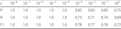
performance. This experiment applies a noiseless sampling method, and two types of experiment data are sampled from above formulas (6) and (7), with-out noise. The iterative times are ten. Both training examples and tested examples are 200. The experi-ment is conducted with a fixed training set and test-ing set method. See the experimental results in Table 1.
Table 1 demonstrates (1) the value of threshold ε, used to judge whether the polynomial value is zero or not, should be small in case of no noise. Because it can be seen from experimental results when ε is small, the values of Precision, Recall, and F1 are all very good, but should not be smaller than machine precision; otherwise, the results cannot be judged. (2) When the threshold ε gradually increases, the per-formance gradually decreases and tends to change monotonously. This shows the VCA method is sensi-tive to the change of threshold in case of no noise, and there is a rule.
3.2.2.2 (b) Experiment with noise The following experiment also aims to verify the impact of the threshold ε, used to judge whether the vanishing component polynomial value is zero or not, on the classification performance, but there is a difference that this experiment adds the Gaussian noise. All ex-perimental data are sampled from above formulas (6) and (7), added with the Gaussian noise μ= 0, σ= 0.1. Both training examples and tested examples are 200. The experiment is conducted under fixed training set and testing set method. See the experimental results in Table 2.
Table 2 demonstrates (1) after adding noise, for the same threshold ε, the experimental performance is lower somewhat than the above experiment without noise. This shows the noise can affect performance. (2) After adding noise, on a whole, the smaller the threshold ε is, the better the performance will be. But under the effect of noise, this result has some excep-tional circumstances. For example, when ε= 10‐1, there is a better result than others. Besides, whenε= 100, the results are not the worst one. This suggests the setting of threshold εis relevant to the features of noise in case
Table 1The impact of the thresholdεof classification decision function in the VCA method on the classification performance (without noise)
ε 10−8 10−7 10−6 10−5 10−4 10−3 10−2 10−1 100
P 1.0 1.0 1.0 1.0 1.0 0.85 0.83 0.83 0.75
R 1.0 1.0 1.0 1.0 1.0 0.73 0.71 0.74 0.69
that noise exists. On the premise of having no idea of noise distribution in advance, it is impossible to set a reasonable value for ε. This directly makes the classification decision function in the VCA method hard to operate.
3.2.3 Problems resulted from over-scaled training set and oversized eigenvector dimension
The influence produced by over-scaled training set and oversized eigenvector dimension: On the one hand, it can be known from the VCA method that the over-scaled training set, i.e., too many training exam-ples, will result in too many vanishing component polynomials, too many monomials contained in the vanishing component polynomial, and too high order of polynomials. Among them, the worst impact is pro-duced by too high order of polynomials. On the other hand, the dimension of eigenvector has a great impact on the computing time of an algorithm, which is be-cause the eigenvector dimension is directly embodied in the number of variables in an algorithm. When there are too many variables, both the number of can-didate polynomial and its maximum number of times will increase rapidly, and the SVD algorithm used to solve zero space will correspondingly quickly become more complex. Both situations will bring about a too long or even intolerable computing time in the VCA method and consequently let the VCA method be less practical.
An experiment against the problem caused by an over-scaled training set: The following experiment aims to directly verify the influence of the order of vanishing component polynomial on the performance and, accord-ingly, indirectly verify the influence of over-scaled train-ing set on the performance. Two types of experimental
data are sampled from the above two groups of polyno-mials, i.e., formulas (6) and (7).
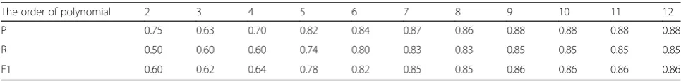
Both the training examples and testing examples are 200. All these 400 examples form an experimental data-set. Having considered that the training sets usually have noise in real situation, the Gaussian noise is set with μ= 0, σ= 0.1. Afterwards, the order of vanishing component polynomial is set as the integer between [2,12]. Then VCA method is used to solve, and the experimental results are as shown in Table3. Table 3indicates that the experimental performance increases with added order of polynomial in the beginning (with the number of times from 2 to 7), but when it reaches to some certain value (with the number of times from 7 to 12), the perform-ance will slowly increase or no longer increase. The reason lies on that a too high order of polynomial may lead to over-fitting phenomena, so that the change of performance goes to a plateau. This proves that too high order of vanishing component polynomial exactly greatly affects the classification performance. Moreover, it can explain over-scaled training set not only increases computation difficulty but also affects the experimental performance.
3.3 GVCA method
According to the abovementioned two problems of the VCA method, i.e., a problem caused by setting thresh-old ε of its classification decision function and a problem resulted from over-scaled training set and oversized eigenvector dimension, this paper proposed a grouping-based VCA (i.e., grouped VCA, abbrevi-ated as GVCA) method to solve the problems. The GVCA method improves the classification decision function in the original VCA method and raises a strategy of grouping training set.
3.3.1 Classification decision function in the GVCA method
The classification decision function in the GVCA method does not preset a thresholdε; instead, it solves the values of all vanishing component polynomials and sorts them (in an order from large to small ac-cording to their absolute values). Later, the top ranked N% = (10%, 20%, 30%,…) ones of all polynomials are selected and judged the class through a majority voting approach. The classification decision function of the GVCA method is as shown in Algorithm 1.
Table 3The influence of the order of vanishing component polynomial in the VCA method on the classification performance
The order of polynomial 2 3 4 5 6 7 8 9 10 11 12
P 0.75 0.63 0.70 0.82 0.84 0.87 0.86 0.88 0.88 0.88 0.88
R 0.50 0.60 0.60 0.74 0.80 0.83 0.83 0.85 0.85 0.85 0.85
F1 0.60 0.62 0.64 0.78 0.82 0.85 0.85 0.86 0.86 0.86 0.86
Table 2The impact of the thresholdεof classification decision function in the VCA method on the classification performance (with noise)
ε 10−8 10−7 10−6 10−5 10−4 10−3 10−2 10−1 100 P 0.88 0.86 0.75 0.75 0.75 0.74 0.78 0.77 0.72
R 0.84 0.81 0.51 0.51 0.60 0.65 0.75 0.76 0.70
This classification decision function has two inputs. One is the vanishing component polynomial set {fn1,…,fnm} of
each class of data produced by training steps via the VCA method, in whichnrepresents the number of class andm represents the number of polynomial corresponding to each class. The other on is the test set Test Data, in which the output is the labels of test set. The main steps are as follows: 5–9: construct double circles with class numbern and testing example number m, respectively, then substi-tute the testing example Test Data into the vanishing component polynomial set {fn1,…,fnm} of each class, and
later figure out the absolute |Valueij| of polynomial value.
10–11: take the top ranked N% results of the calcu-lated absolute value |Valueij| of vanishing
compo-nent polynomial and choose the class of maximum amount as the class label of testing example.
3.3.2 Training set grouping strategy in the GVCA method
(1) Grouping the training set: this paper proposed the GVCA method to address two situations of over-scaled training set and too high dimension of eigenvector. Regarding the problem of over-scaled training set, it is a practicable way to group the examples, i.e., to horizontally segment the entire training set into several training subsets (for instance, take 10/20/30/40/50 examples as a group), then acquire the features (i.e., vanishing component polynomial) by the original VCA method respectively and combine the vanishing component polynomial in multiple grouped training sets into the vanishing component polynomial in an integral training set. This approach is called the horizontal grouping method.
The GVCA method based on horizontally grouped training set is as shown in Algorithm 2. Meanwhile, regarding the problem of too high eigenvector dimen-sion of training set, a feasible approach is to group
(2) Prove the correctness of the strategy of grouping training set: the following paragraphs expound and prove the correctness of the strategy of grouping training set in the GVCA method. There are vertically and horizontally grouping cases, stated respectively below.
3.3.2.1 (a) Horizontal grouping In nature, the VCA method lies on doing feature mapping x→jpl
jðxÞj on
dataset, i.e., mapping the dataset forx into a dataset for t¼ ðjp11ðxÞj;…;jplnlðxÞjÞ, in which, fpl1ðxÞ;…;plnlðxÞg is the generator for vanishing ideal of class l. Horizontally grouping the training set is equivalent to Bagging inte-grated learning implemented after bootstrap sampling ont. Due to the correspondence between Grobner basis and dataset x, the results of classifyingt can be directly mapped back tox, thus guaranteeing its correctness.
3.3.2.2 (b) Vertical grouping Vertical grouping is equivalent to attribute Bagging done tot, which means to repeatedly sample the eigenvector set to obtain the feature subsets. Either group is allowed to cross each other, in other words, different feature subsets are allowed to con-tain several same features. In accordance with the theory raised in [39], its correctness can be ensured as well.
(3) Analysis on time complexity of grouped training set: Assume the size of training set isMbefore being grouped, and the dimension of eigenvector is
N. From the original VCA method, the following conclusions [4] can be obtained:
(a) The training under the VCA method will finish after iteration fort≤M+ 1 times at the most. (b) The highest order of polynomial in both non-vanishing
component polynomial setFand vanishing component polynomial setVareMorder at the most.
(c) |F|≤M, and|V|≤|F|2× min {|F|,N}.
(d) The time complexity of all vanishing component polynomial inVis computed to beO(|F|2+ |F| × |V|).
Before grouping the training set, usually M〉〉N; there-fore, the time complexity of all vanishing component polynomial inVis computed to be:
O Fj j2þj j F j jV≤O M 2þMj jV
≤O M 2þMj jF2 min Ffj j;Ng ≤O M 2þMM2 min Mf ;Ng
≤O M 2þMM2N
¼O M 2þM3N
ð8Þ According to formula (8), it can be known that the time complexity of non-grouped training set is:
O M 3N ð9Þ
Now, the training set is segmented into kgroups that do not intersect, and the example number of each group is m, so it is easily known that M=km. Besides, the eigenvector dimension is tillN, and after grouping, usually m≤N. Therefore, the time complexity of all vanishing component polynomial in each subgroupVi,i= 1,…,kis
computed to be:
O Fj ji2þj j Fi j jVi
≤O m2þmj jVi
≤O m2þmj jFi2 min Ffj j;i Ng
≤O m 2þmm2 min mf ;Ng
≤O m 2þmm2m¼O m4
ð10Þ
According to formula (10), it can be known that the time complexity of grouped training set is:
O k m4 ð11Þ
In addition, due toM=km, the total time complexity of grouped training set is
O k m4¼O k ðM=kÞ4¼O M 4=k3 ð12Þ
Then, according to formulas (9) and (12), the ratio of time complexity before and after grouping training set is
M4=k31=M3N¼M=k3N ð13Þ
It is known from formula (13) that, when the grouping number k is large enough, the ratio of time complexity before and after grouping training set will be small enough. However, as the value ofkcan beMat the most (in real situation, it should be a suitable value approxi-mating toM), so the minimal value of such ratio will be:
M=k3N≥M=M3N¼1=M2N ð14Þ
The formula (14) is the lower bound of such ratio. Example 1. Suppose the size of training set before be-ing grouped is M= 1000, the eigenvector dimension is N= 100, the training set is segmented intok= 20 groups, and the size of training set in each group is m= 50. It can be seen from formula (13) that the time complexity of grouped training set has been reduced to the follow-ing ratio of that before groupfollow-ing.
M=k3N¼1000=203100¼10=203
¼1=800 ð15Þ
4 Results and discussion
This paper had totally designed and completed four groups of experiments. At first, by experiment, it found out a proportion of sorted vanishing component polyno-mial suited to the classification decision function in the GVCA method. Next, by experiment, it found out a suit-able size of grouped training set (including horizontally and vertically). At last, on the basis of the above two ex-periments, the classification and convergence perform-ance of the GVCA method were tested on simulation dataset and UCI dataset, respectively.
4.1 Experimental settings
The data used in simulation dataset were sampled from the abovementioned formulas (6) and (7), with all exam-ples added with Gaussian noise atμ= 0,σ= 0.02(σ= 0.06,
σ= 0.1). In order to generate balanced vanishing compo-nent polynomial, the number of two classes of examples was set to be equal.
The UCI standard dataset is a dataset for machine learning proposed by the University of California, Irvine. It is a frequently used standard testing dataset. Depending on the experimental need, the paper chose two types of data subsets in UCI dataset. One is a dataset with small eigenvector dimension, which includes seven subdatasets such as Wine, Transfusion, Connectionist Bench, Breast Cancer Wisconsin, Indian Liver Patient, Mammographic
Masses, and Iris. The dataset scale and eigenvector dimen-sion are as shown in Table4.
And the other one is a dataset with large eigenvector dimension, which includes seven subdatasets such as Onehr, Hill Valley(with noise and without noise), LSVT, and 100Plant Species(data Sha 64, data Tex 64 and data Mar 64). The subset scale and attribute dimension are as shown in Table5. Their universality lies on their be-ing classification task, full data type, small scaled train-ing set, and convenient to test. Other classification algorithms chosen to compare with the GVCA method involves the decision tree, naive Bayesian classifier, K-neighborhood, SVM (polynomial kernel), and SVM (Gaussian kernel). All of them are commonly used clas-sification algorithm with good performance. Using Weka [40] as the experimental platform, the compari-son was made until the performance had been regu-lated to a good state through a parameter selection method [41] in the experiment. In view of possible de-fault in some certain data, the decision tree J48 algo-rithm was used together with Laplace smoothing method. The K-neighborhood employed IBk algorithm and set the neighborhood parameter to be 7. The SVM used SMO algorithm, and considering the computa-tional complexity, the exponent parameter of polyno-mial kernel was set to be 2, and the gamma parameter of Gaussian kernel was set as 0.01.
4.2 An experiment studying the influence of the proportion of vanishing component polynomial of classification decision function in the GVCA method on the classification performance
Likewise, the paper used the following experiment to verify the rationality of classification decision function in Table 4UCI dataset used in the experiment
Dataset Example no. Eigenvector Classification no.
Wine 178 13 3
Transfusion 748 5 2
Connectionist Bench 528 10 10
Breast Cancer Wisconsin 699 10 2
Indian Liver Patient 583 10 2
Mammographic Masses 961 6 2
Iris 150 4 3
Table 5UCI dataset used in the experiment
Dataset Example no. Eigenvector Classification no.
Onehr 2536 73 2
LSVT 126 309 2
Hill Valley (with noise) 606 100 2
Hill Valley (without noise) 606 100 2
100Plant Species (data Sha 64)
1600 64 100
100Plant Species (data Tex 64)
1600 64 100
100Plant Species (data Mar 64)
1600 64 100
Table 6The influence of the sorting-purpose polynomial proportion in classification decision function of the GVCA method on the classification performance
N% 10% 20% 30% 40% 50% 60% 70% 80% 90%
P 0.83 0.84 0.86 0.88 0.86 0.86 0.86 0.88 0.87
R 0.76 0.80 0.81 0.84 0.83 0.83 0.83 0.86 0.84
F1 0.79 0.82 0.83 0.85 0.84 0.84 0.84 0.86 0.85
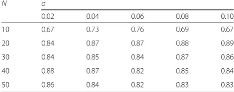
Table 7The influence of the horizontal grouping of simulation dataset in the GVCA method on the classification performance
N σ
0.02 0.04 0.06 0.08 0.10
10 0.67 0.73 0.76 0.69 0.67
20 0.84 0.87 0.87 0.88 0.89
30 0.84 0.85 0.84 0.87 0.86
40 0.88 0.87 0.82 0.85 0.84
the proposed GVCA method. The experiment aims to examine the influence of sorting-purpose polynomial proportion on the performance. In the experiment, the results of polynomial were sorted in an order from small to large according to their absolute values, and then the class with the maximum numbers in top ranked N% of the total number was determined as the class label. The experimental results are as shown in Table6. This indicates when N% increases to a certain quantity, specifically in this table, when N% = 20% until N% = 70%, the experimental performance re-mains stable. WhenN% = 80%, the performance turns to be better yet with limited superiority. So, there is a stable interval from 20 to 70% in the number of van-ishing component polynomial required to sort in classification decision function of the GVCA method. During this range, there is no large change in perform-ance. For this reason, the proportion of sorted vanish-ing component polynomial adopted in this paper is N% = 20%.
4.3 Experiments studying the influence of the size of grouped training set in the GVCA method on the classification performance
A. An experiment conducted on simulation dataset An experiment was conducted on simulation dataset to study the relation between the size of grouped training set and the classification performance. Firstly, this paper used a simulation dataset and sampled all experimental data from the above formulas (6) and (7), with all examples added with Gaussian noise atμ= 0,σ= 0.02, σ= 0.04, …,
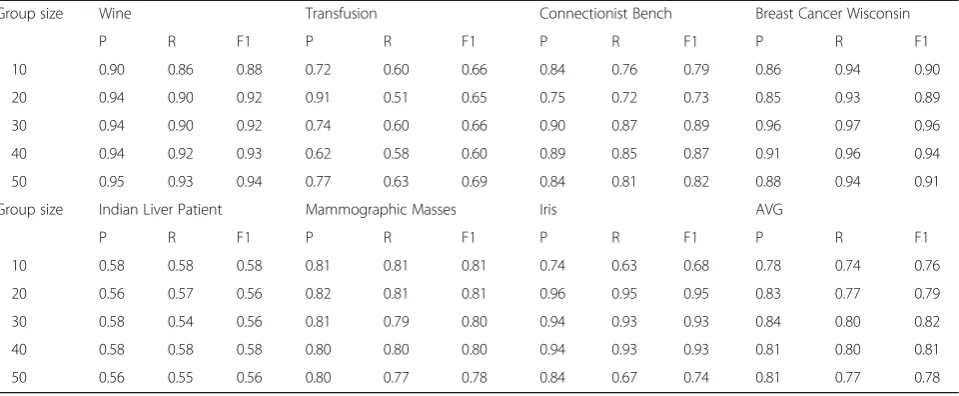
σ= 0.10. In order to generate balanced vanishing compo-nent polynomial, the number of two classes of examples was set to be equal. Due to small eigenvector dimension in simulation dataset, only horizontal grouping experi-ment was impleexperi-mented. The size of horizontally grouped training set was set as 10/20/30/40/50. The experimental results are as shown in Table7, in which,Nrepresents the size of grouped dataset, and the experimental performance is represented by F1 value corresponding to differentσ. It can be known from Table 7 that, though the values Table 8The influence of the horizontal grouping of UCI dataset in the GVCA method on classification performance
Group size Wine Transfusion Connectionist Bench Breast Cancer Wisconsin
P R F1 P R F1 P R F1 P R F1
10 0.90 0.86 0.88 0.72 0.60 0.66 0.84 0.76 0.79 0.86 0.94 0.90
20 0.94 0.90 0.92 0.91 0.51 0.65 0.75 0.72 0.73 0.85 0.93 0.89
30 0.94 0.90 0.92 0.74 0.60 0.66 0.90 0.87 0.89 0.96 0.97 0.96
40 0.94 0.92 0.93 0.62 0.58 0.60 0.89 0.85 0.87 0.91 0.96 0.94
50 0.95 0.93 0.94 0.77 0.63 0.69 0.84 0.81 0.82 0.88 0.94 0.91
Group size Indian Liver Patient Mammographic Masses Iris AVG
P R F1 P R F1 P R F1 P R F1
10 0.58 0.58 0.58 0.81 0.81 0.81 0.74 0.63 0.68 0.78 0.74 0.76
20 0.56 0.57 0.56 0.82 0.81 0.81 0.96 0.95 0.95 0.83 0.77 0.79
30 0.58 0.54 0.56 0.81 0.79 0.80 0.94 0.93 0.93 0.84 0.80 0.82
40 0.58 0.58 0.58 0.80 0.80 0.80 0.94 0.93 0.93 0.81 0.80 0.81
50 0.56 0.55 0.56 0.80 0.77 0.78 0.84 0.67 0.74 0.81 0.77 0.78
Table 9The influence of the vertical grouping of UCI dataset in the GVCA method on classification performance
Group number Wine Transfusion Connectionist Bench Breast Cancer Wisconsin
P R F1 P R F1 P R F1 P R F1
2 0.90 0.88 0.89 0.92 0.73 0.81 0.76 0.82 0.79 0.91 0.90 0.90
3 0.89 0.92 0.90 0.87 0.79 0.83 0.86 0.85 0.85 0.89 0.87 0.88
4 0.86 0.90 0.88 0.76 0.80 0.78 0.87 0.89 0.88 0.91 0.85 0.88
Group number Indian Liver Patient Mammographic Masses Iris AVG
P R F1 P R F1 P R F1 P R F1
2 0.86 0.87 0.86 0.87 0.87 0.87 0.92 0.90 0.91 0.83 0.77 0.79
3 0.85 0.86 0.85 0.83 0.80 0.81 0.90 0.93 0.91 0.84 0.80 0.82
of standard deviationσare varied, the optimum experi-mental performance appears under a moderate scale of grouped dataset (that isN= 20 toN= 40, in this table). The reason of this phenomenon is the undersized or oversized scale of grouped dataset will result in under-fitting or over-under-fitting.
B. An experiment conducted on UCI dataset
Below, UCI standard dataset was chosen to study the influence of the size of grouped training set in the GVCA method on the classification performance.
Horizontal grouping means to group the dataset ex-ample. The paper tested seven subdatasets contained in UCI standard dataset, such as Wine, Transfusion, Con-nectionist Bench, Breast Cancer Wisconsin, Indian Liver Patient, Mammographic Masses, and Iris. The number of grouped dataset was 10/20/30/40/50, respectively. The evaluation criterion was set as Precision, Recall, and F1. After several tests, the performance of different training sets was averaged, see results in Table 8. This set of experimental results shows a total trend: when the
grouped scale in the GVCA method is placed in a mid-dle position, that is, taking 30 or 40 examples to com-pose one subgroup, the obtained performance will be the best. And the performance may slightly decrease with a lower or higher value than 30 and 40. The reason for this is when the grouping scale is moderate, neither under-fitting nor over-fitting will happen. Therefore, the GVCA method can acquire an optimum performance in the vertical grouping test.
Vertical grouping means to group the eigenvector di-mension. After several tests, the performance of different training sets was averaged, see results in Table9.
4.4 Experiments comparing the performance of the GVCA method and other classification algorithms
4.4.1 An experiment conducted on simulation dataset
This paper utilized simulation dataset to compare the GVCA method with other classification algorithms. The experimental data were still sampled from the above for-mulas (6) and (7), with all examples added with Gauss-ian noise at μ=0,σ=0.02(σ=0.06,σ=0.1). The training set used 10, 20, 30, 40, 50, 100, 150, and 200 examples, re-spectively. The machine learning methods for contrast are decision tree, naive Bayesian classifier, K-neighborhood, SVM (polynomial kernel), and SVM (Gaussian kernel). The evaluation criterion was set as Precision, Recall, and F1. After several tests, the results of different training set sizes were averaged, see results in Table10, in which DT represents naive Bayesian clas-sifier, KNN represents K-neighborhood, POLYK repre-sents SVM (polynomial kernel), and RBFK reprerepre-sents Table 10Comparison of the classification performance on
simulation dataset by the GVCA method and other classification algorithms
Algorithm Precision Recall F1
DT 0.90 0.88 0.89
NB 0.87 0.84 0.85
KNN 0.83 0.76 0.79
POLYK 0.78 0.65 0.71
RBFK 0.76 0.72 0.74
GVCA 0.94 0.92 0.93
Table 11Comparison of the classification performance on UCI dataset by the GVCA method and other classification methods
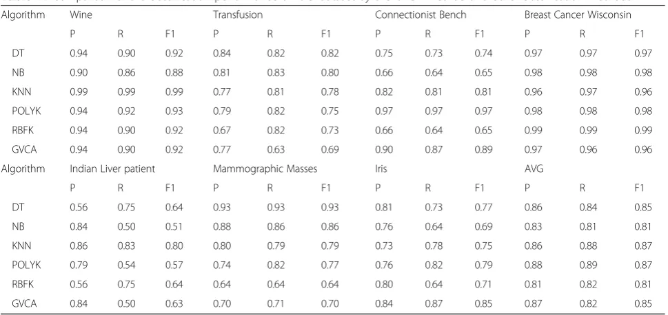
Algorithm Wine Transfusion Connectionist Bench Breast Cancer Wisconsin
P R F1 P R F1 P R F1 P R F1
DT 0.94 0.90 0.92 0.84 0.82 0.82 0.75 0.73 0.74 0.97 0.97 0.97
NB 0.90 0.86 0.88 0.81 0.83 0.80 0.66 0.64 0.65 0.98 0.98 0.98
KNN 0.99 0.99 0.99 0.77 0.81 0.78 0.82 0.81 0.81 0.96 0.97 0.96
POLYK 0.94 0.92 0.93 0.79 0.82 0.75 0.97 0.97 0.97 0.98 0.98 0.98
RBFK 0.94 0.90 0.92 0.67 0.82 0.73 0.66 0.64 0.65 0.99 0.99 0.99
GVCA 0.94 0.90 0.92 0.77 0.63 0.69 0.90 0.87 0.89 0.97 0.96 0.96
Algorithm Indian Liver patient Mammographic Masses Iris AVG
P R F1 P R F1 P R F1 P R F1
DT 0.56 0.75 0.64 0.93 0.93 0.93 0.81 0.73 0.77 0.86 0.84 0.85
NB 0.84 0.50 0.51 0.88 0.86 0.86 0.76 0.64 0.69 0.83 0.81 0.81
KNN 0.86 0.83 0.80 0.80 0.79 0.79 0.73 0.78 0.75 0.86 0.88 0.87
POLYK 0.79 0.54 0.57 0.74 0.82 0.77 0.76 0.82 0.79 0.88 0.89 0.87
RBFK 0.56 0.75 0.64 0.64 0.64 0.64 0.80 0.64 0.71 0.81 0.82 0.81
SVM (Gaussian kernel). It can be discovered from Table 10 that the average performance of the GVCA method is higher than other five machine learning methods.
4.4.2 An experiment conducted on UCI dataset
This paper tested seven subdatasets contained in UCI standard dataset, such as Wine, Transfusion, Connec-tionist Bench, Breast Cancer Wisconsin, Indian Liver Patient, Mammographic Masses, and Iris. The evalu-ation criterion was set as Precision, Recall, and F1. After several tests, the performance of different training sets were averaged, see results in Table 11. These re-sults indicate that compared to some classification al-gorithms, the proposed the GVCA method can achieve perfect average performance, which fully displays its strong stability and perfect performance.
4.5 Experiments comparing the convergence rate by the GVCA method and other classification algorithms
The following experiments aim to test the convergence performance by the GVCA method. For simulation dataset and UCI dataset, the 25, 30, 35, 40, 45, 50, and 55% of total example number were adopted as the training set, and the balanced ones were taken as test-ing set and compared with common machine learntest-ing methods. The evaluation indexes are F1 values corre-sponding to different training set scales and different classification algorithms.
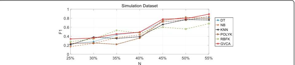
4.5.1 An experiment conducted on simulation dataset
After several tests, the performance of different training sets was averaged, see results in Fig.1.
4.5.2 An experiment conducted on UCI dataset
The paper tested the convergence rate of seven subda-tasets contained in UCI standard dataset, such as Wine, Transfusion, Connectionist Bench, Breast Cancer Wisconsin, Indian Liver Patient, Mammographic Masses, and Iris. The experimental results are as shown in Fig.2, which indicates the GVCA method can still obtain a good performance with a small training set scale (less than 50%) compared to other methods. This is because the Grobner basis acquired by the GVCA method on a moderate-scale grouped training set could well characterize the inner structure of a manifold pattern. Thus, the GVCA method can get a rapid rate of convergence and quickly achieve favorable learning performance.
5 Conclusions
This paper analyzed the characteristics and existing problems of the VCA method, and then improved it from both aspects to form a GVCA method. (1) The classification decision function is based on the sorting of values that vanishing components take from tested data, while the non-vanishing component makes its decision depending on the number of value being zero taken from tested data. This avoids the problem of not easily set threshold of classification decision function for the VCA method and enhances feasibility in real application. Fig. 1Comparison of the convergence rate of simulation dataset by the GVCA method and other classification algorithms
(2) A strategy of grouping training set was proposed, which segmented training set into several non-intersecting sub-sets, solved the vanishing polynomial on subset, and com-bined them into the vanishing component polynomial set of an integral training set, to apply to solve the problem of large-scaled training set. (3) The integrated learning theory was utilized to prove the correctness of the strategy of grouping training set. The analysis of time complexity be-fore and after grouping demonstrates it can effectively re-duce computational time. A series of experimental results show that the GVCA method obtains a perfect experimen-tal performance and quicker convergence compared to other classification algorithms.
In future, the dual relation between ideal space and kernel space can be further used to switch the computation of kernel space into that of ideal space, thereby realizing the application of commutative algebra to efficiently solve the machine learning problem.
Abbreviation
AVICA:Approximate vanishing ideal component analysis; DT: Decision tree; GVCA: Grouped vanishing component analysis; IPCA: Ideal principal component analysis; Kernel PCA: Kernel primary component analysis; KNN: K-nearest neighbor; NB: Naive Bayesian; PCA: Principal component analysis; POLYK: Support vector machine with polynomial kernel; RBFK: Support vector machine with Gaussian kernel; SD: Stochastic discrimination; SVD: Singular value decomposition; SVM: Support vector machine; UCI: University of California Irvine; VCA: Vanishing component analysis
Author’s contributions
XZ is the writer of this paper. He proposed the main idea, deduced the performance of the GVCA method, completed the simulation, and analyzed the result. The author read and approved the final manuscript.
Competing interests
The author declares that he has no competing interests.
Publisher’s Note
Springer Nature remains neutral with regard to jurisdictional claims in published maps and institutional affiliations.
Received: 7 March 2018 Accepted: 18 April 2018
References
1. D Eisenbud, Commutative algebra: With a view toward algebraic geometry. Springer Science & Business Media150(2013)
2. M. Waldschmidt,“Diophantine Approximation and Diophantine Equations,”2011. 3. JB Tenenbaum, V De Silva, JC Langford, A global geometric framework for
nonlinear dimensionality reduction. Science90(5500), 2319–2323 (2000) 4. R Livni, D Lehavi, S Schein, H Nachliely, S Shalev-Shwartz, A Globerson, in
Proceedings of The 30th International Conference on Machine Learning. Vanishing component analysis (2013), pp. 597–605
5. D Lazard, inComputer algebra. Gröbner bases, Gaussian elimination and resolution of systems of algebraic equations (Springer, 1983), pp. 146–156 6. N Cristianini, J Shawe-Taylor,An introduction to support vector machines and
other kernel-based learning methods(Cambridge University Press, 2000) 7. CM Bishop et al.,Pattern recognition and machine learning, vol 4 (Springer,
New York, 2006), p. no. 4
8. CF Gauss,Disquisitiones arithmeticae, vol 157 (Yale University Press, 1966) 9. EE Kummer,De numeris complexis, qui radicibus unitatis et numeris integris
realibus constant(Gratulationsschrift der Univ. Breslau in Jubelfeier der Univ., Königsberg, 1844), pp. 185–212
10. R Dedekind,Theory of Algebraic Integers(Cambridge University Press, 1996) 11. R Courant, D Hilbert,Methods of mathematical physics, vol 1 (CUP Archive, 1966)
12. S Lang,Algebraic number theory, vol 110 (Springer Science & Business Media, 2013)
13. B Stenström,Rings of quotients: An introduction to methods of ring theory, vol 217 (Springer Science & Business Media, 2012)
14. G Dedekind,“Belt press apparatus with heat shield,”Jun. 22 1982, uS Patent 4,336,096.
15. MF Atiyah, IG Macdonald,Introduction to commutative algebra, vol 2 (Addison-Wesley Reading, 1969)
16. GE Noether,On a theorem of pitman(The Annals of Mathematical Statistics, 1955), pp. 64–68
17. N Bourbaki,Algebra I: chapters 1–3(Springer Science & Business Media, 1998) 18. CA Weibel,An introduction to homological algebra(Cambridge university
press, 1995), p. no. 38
19. O Endler, W Krull,Valuation Theory(Springer, 1972)
20. HM Möller, B Buchberger,The construction of multivariate polynomials with preassigned zeros(Springer, 1982)
21. D Heldt, M Kreuzer, S Pokutta, H Poulisse, Approximate computation of zero-dimensional polynomial ideals. J. Symb. Comput.44(11), 1566–1591 (2009) 22. GH Golub, CF Van Loan,Matrix computations, vol 3 (JHU Press, 2012) 23. RM Corless, PM Gianni, BM Trager, SM Watt, inProceedings of the 1995
international symposium on Symbolic and algebraic computation. The singular value decomposition for polynomial systems (ACM, 1995), pp. 195–207 24. HJ Stetter,Numerical polynomial algebra(Siam, 2004)
25. NJ Higham,Accuracy and stability of numerical algorithms(Siam, 2002) 26. AM Garsia, Combinatorial methods in the theory of Cohen-Macaulay rings.
Adv. Math.38(3), 229–266 (1980)
27. T Sauer, Approximate varieties, approximate ideals and dimension reduction. Numerical Algorithms45(1–4), 295–313 (2007)
28. F J. Király, M. Kreuzer, and L. Theran,“Dual-to-kernel learning with ideals,” arXiv preprint arXiv:1402.0099, 2014.18.
29. S Mika, B. Schölkopf, A. J. Smola, K.-R. Müller, M. Scholz, and G. Rätsch,
“Kernel pca and de-noising in feature spaces.”in NIPS, vol. 4, no. 5. Citeseer, 1998, p. 7.
30. E Kleinberg,Stochastic discrimination(Annals of Mathematics and Artificial Intelligence, 1990)
31. TK Ho, The random subspace method for constructing decision forests. IEEE Trans. Pattern Anal. Mach. Intell.20(8), 832–844 (1998)
32. LK Hansen, P Salamon, Neural network ensembles. IEEE Trans. Pattern Anal. Mach. Intell.12(10), 993–1001 (1990)
33. L Breiman,Bagging predictors(Machine Learning, 1996) 34. RE Schapire,“A brief introduction to boosting,”1999.
35. RE Schapire, Y Freund, P Bartlett, WS Lee, Boosting the margin: A new explanation for the effectiveness of voting methods. Ann. Stat.26(5), 1651–1686 (1998)
36. S Cho, JH Kim, Multiple network fusion using fuzzy logic. IEEE Trans. Neural Netw.6(2), 497–501 (1995)
37. DH Wolpert, Stacked generalization. Neural Networks5(2), 241–259 (1992) 38. WVD Hodge, W Hodge, D Pedoe,Methods of algebraic geometry, vol 2
(Cambridge University Press, 1994)
39. WW Adams, P Loustaunau,An introduction to Grobner bases(American Mathematical Soc., 1994)
40. R Bryll, R Gutierrezosuna, F Quek, Attribute bagging: Improving accuracy of classifier ensembles by using random feature subsets. Pattern Recogn.36(6), 1291–1302 (2003)
41. M Hall, E Frank, G Holmes, B Pfahringer, P Reutemann, IH Witten, The Weka data mining software: An update. ACM SIGKDD explorations newsletter