An expanded mixed finite element simulation for two sided time dependent fractional diffusion problem

(1)

R E S E A R C H

Open Access

An expanded mixed ﬁnite element

simulation for two-sided time-dependent

fractional diffusion problem

Qiong Yuan and Huanzhen Chen

*

*_{Correspondence:} [email protected] School of Mathematics and Statistics, Shandong Normal University, Jinan, China

Abstract

In this paper, we consider a time-dependent diffusion problem with two-sided Riemann-Liouville fractional derivatives. By introducing a fractional-order flux as auxiliary variable, we establish the saddle-point variational formulation, based on which we employ a locally conservative mixed finite element method to approximate the unknown function, its derivative and the fractional flux in space and use the backward Euler scheme to discrete the time derivative, and thus propose a fully discrete expanded mixed finite element procedure. We prove the well-posedness and the optimal order error estimates of the proposed procedure for a sufficiently smooth solution. Numerical experiments are presented to confirm our theoretical findings.

Keywords: time-dependent fractional diﬀusion problem; expanded mixed ﬁnite

element method; fully discrete scheme; well-posedness; error estimates

1 Introduction

We consider the following time-dependent fractional diﬀusion equation of order 2 –β:

(a) ∂u ∂t –D

Kθ0Ixβ+ (1 –θ)xI

β

1

Du(x,t) =f(x,t), x∈,t∈(0,T],

(b) u(x, 0) =u0, x∈,

(c) u(0,t) =u(1,t) = 0, t∈[0,T],

(1.1)

where= (0, 1), 0 <β< 1, 0≤θ≤1,Kis the diﬀusivity coeﬃcient andf ∈L2₍_{) is the}

source or sink term;D= ∂

∂xis the ﬁrst-order derivative operator,0I

β

x andxI

β

1 represent the

left and right fractional integral operators of orderβ, respectively, defined by (2.1). The interest in (1.1) is motivated by its application to physical phenomena. Numerous experiments show that fractional diffusion equations have more advantages and higher accuracy in modeling anomalous or non-Fickian diffusion processes that arise from tur-bulent flow [1, 2], chaotic dynamics [3] and viscoelasticity [1]. Recently, a series of defi-nition of the fractional derivative were proposed [4–6]. These new defidefi-nitions can better describe the chemical kinetics system pertaining [7], the generation of nonlinear water-waves in the long-wavelength regime [8], the convective straight fins with temperature-dependent thermal conductivity [9], the relaxation and diffusion models [4], optimal

(2)

trol problems [5], the motion of a bead sliding on a wire [10], the material heterogeneities and structures with diﬀerent scales [6].

In general, Fourier transform and Laplace transform are useful tools to obtain the an-alytic solutions of fractional partial differential equations. However, these two methods are available only in a few limited cases. Thus, it is important to find practical numeri-cal means to deal with fractional model. In the last decade, different numerinumeri-cal methods have been developed, such as the difference method [11, 12], the spectral method [13], the fast difference method [14], the finite volume method [15, 16], the homotopy analy-sis transform method [17, 18], the efficient nonstandard finite difference method [19], the Riesz-Caputo difference method [20], and the Riesz-Riemann-Liouville difference method [21].

Galerkin finite element method is another way to solve fractional derivative equations. In the series of works [22–24], Ervin and Roop presented a first rigorous analysis for the stationary fractional advection dispersion equation based on a variational formulation. Then the discontinuous Galerkin method [25], mixed finite element method [26–30], Petrov Galerkin method [31] and the least-squared mixed method are proposed [32] for stationary fractional diffusion equations, consecutively.

In this article, we employ an expanded mixed finite element to discrete fractional diffu-sion part and use the backward Euler scheme to approximate the time derivative, and thus propose a fully discrete procedure for the time-dependent fractional diffusion equation (1.1). The solvability and stability of the fully discrete scheme is proved and the optimal-order numerical analysis are presented. Numerical experiments are conducted to verify our theoretical findings.

This paper is organized as follows. In Section 2, we recall preliminaries on fractional calculus and present the equivalent relations among negative fractional derivative spaces, fractional derivative spaces and the standard Sobolev spaces. In Section 3, by introduc-ing the ﬂux functionp= –K(θ0Iβx + (1 –θ)xI1β)Duandq=Duwe derive the corresponding

saddle-point formulation and the locally conservative expanded mixed ﬁnite element pro-cedure, with its well-posedness analyzed. Optimal-order error analysis for fully regular solution would be given in Section 4 and numerical experiments are performed to verify our theoretical results in Section 5. In Section 6, some concluding remarks are presented.

2 Preliminaries

We first briefly revisit the definitions and some properties of left-sided and right-sided Riemann-Liouville fractional derivatives.

Letμ> 0,0Ixμbe the left-sided fractional integral operator of orderμ, deﬁned by

0Ixμu= 1 (μ)

x

0

(x–s)μ–1u(s)ds, (2.1)

where(·) is the Gamma function. Based on the deﬁnition of integral operator, we in-troduce the left-sided Riemann-Liouville fractional derivative of orderμin [33–35]. Let n∈N+_satisfy_n_{– 1 <}_μ_<_n_{, then}

0Dμxu=

dn

dxn

0Ixn–μu

(3)

Similarly, the right versions of fractional-order integral and derivative are deﬁned as

xI1μu=

1 (μ)

1

x

(s–x)μ–1u(s)ds (2.3)

and

xDμ1u= (–1)n

dn dxn

xI1n–μu

. (2.4)

The fractional integral operator0IxandxI1satisfy the semigroup property

0Ixν+μu=0Ixν0Ixμu,

xI1ν+μu=xIν1xI1μu, for allu∈L2()

(2.5)

and the adjoint property

0Ixμu,v

=u,xI1μv

, for allu,v∈L2(). (2.6)

The left fractional derivative spaces J_Lμ_,0() [23] are deﬁned as the closure ofC₀∞() under the norms · _Jμ

L

|u|_Jμ

L():=0D

μ

xuL2₍₎,

u_Jμ

L():=

u2_L2₍₎+|u|2_Jμ

L()

1/2

.

The right fractional derivative spacesJ_Rμ_,0() are deﬁned similarly. In these spaces, the fractional diﬀerential operators satisfy the semigroup property [23]

0Dμxu=0Dνx0Dμx–νu, for allu∈J

μ

L,0(). (2.7)

The equivalence theory for the fractional derivative spaces is described by the following lemma.

Lemma 2.1([23], Theorem 2.13) Letμ> 0andμ=n–₂1,n= 1, 2, . . . .Then the J_Lμ_,0()and J_Rμ_,0()are equal to the fractional-order Sobolev space H₀μ(),with equivalent semi-norms and norms.

Parallel to Lemma 2.1, we shall deﬁne the negative fractional derivative spaces and es-tablish their equivalence theory with the negative fractional-order Sobolev spaces.

The left negative fractional derivative spacesJ_L–μ() [36] are deﬁned as the closure of C₀∞() under the norms · _J–μ

L

u_J–μ

L ():=0I

μ

xuL2₍₎.

(4)

Lemma 2.2([36], Theorem 2.6) Letμ> 0,μ=n–1₂,n= 1, 2, 3, . . . .Then the negative fractional spaces J_L–μ()and J_R–μ()are equal to the standard negative fractional Sobolev space H–μ₍₎_{with equivalent norms}_._Furthermore_,

0Ixμv,xI

μ

1v

=cos(μπ)v2_H–μ₍₎. (2.8)

For simplicity, we only use·μ,|·|μor·–μto represent their norms and semi-norms

in the following sections. Whenμ= 0, we understandH0₍_{) =}_L2₍_{) and simply use}_·

to denote its norm.

We also need the deﬁnition of Sobolev spaces involving time deﬁned by, for any Banach spaceX,

W_qm(t1,t2;X) :=

f(x,t) :∂

α_f

∂tα(·,t)

X

∈Lq(t1,t2), 0≤α≤m, 1≤q<∞ ,

fWm

q(t1,t2;X):= ⎧ ⎨ ⎩

(m_α₌₀t2

t1

∂αf

∂tα(·,t)

q Xdt)

1

q_, ₁≤_q_<∞_,

max0≤α≤messsupt∈(t1,t2)

∂αf

∂tα(·,t)X, q=∞. We conclude this section by the following commonly used inequality.

Lemma 2.3(Discrete Gronwall inequality) Lett,B,C> 0, (an)n, (bn)n, (cn)n, (dn)nbe

sequence of nonnegative numbers satisfying

an+t n

i=0

bi≤B+Ct n

i=0

ai+t n

i=0

ci, ∀n≥0.

Then,if Ct< 1,we have

an+t n

i=0

bi≤eC(n+1)t

B+t

n

i=0

ci

, ∀n≥0.

3 Mixed ﬁnite element procedure

We begin this section by introducing the intermediate variableq,pand rewrite (1.1) into the following saddle-point problem:

(a) q=Du, x∈,

(b) p= –Kθ0Ixβ+ (1 –θ)xI1β

q, x∈,

(c) ut+Dp=f, x∈,

(d) u(x, 0) =u0.

(3.1)

We letV:=H1₍_),_H_:=_H–β2₍_{) and}_W_:=_L2₍_{). In order to deﬁne the variational}

(5)

(3.1) or (1.1) as to ﬁnd (p,q,u)∈V×H×Wsuch that

(a) (q,v) + (u,Dv) = 0, ∀v∈V,

(b) (p,σ) +Kθ0Ixβ+ (1 –θ)xI1β

q,σ= 0, ∀σ∈H,

(c) (ut,w) + (Dp,w) = (f,w), ∀w∈W,

(d) u(x, 0) =u0.

(3.2)

Based on the saddle-variational formulations (3.2), we shall construct a fully discrete mixed ﬁnite element scheme for the fractional diﬀusion equation(1.1).

Let us uniformly divide = [0, 1] byIi= [xi–1,xi], i= 1, 2, . . . ,Mwith x0= 0,xM= 1,

h=xi–xi–1. Lettn=nτ, n= 0, 1, . . . ,J, whereτ =T/J is time step. We denote Raviart-Thomas spaces or Brézzi-Douglas-Marini spaces [28, 37–39] byVh×Wh⊂V×W with space indexk≥0 andHh⊂His a piecewise ﬁnite dimensional subspace deﬁned by

Vh=

vh∈V;vh|Ii∈Pk+1(Ii),k≥0

,

Hh=

σh∈H;σh|Ii∈Pk+1(Ii),k≥0

,

Wh=

wh∈W;wh|Ii∈Pk(Ii),k≥0

.

(3.3)

HerePk(Ii) is the restriction of all polynomials of degree not bigger thanktoIi.

We use the backward Euler scheme to discrete the time derivative of first order and define the fully discrete mixed finite element procedure of (3.2) so as to find (pn_h,qn_h,un_h)∈ Vh×Hh×Whsuch that

(a) q_hn,vh

+un_h,Dvh

= 0, ∀vh∈Vh,

(b) pn_h,σh

+Kθ0Ixβ+ (1 –θ)xI1β

qn_h,σh

= 0, ∀σh∈Hh,

(c)

un h–unh–1

τ ,wh

+Dpn_h,wh

=fn,wh

, ∀wh∈Wh,

(d) u0_h=Rhu0.

(3.4)

We assume

Vh=span{ϕi}Ni=1+1, Hh=span{ϕj}Nj=1+1, Wh=span{φk}Lk=1,

and expresspn

h,qnh,unhas

pn_h= N+1

i=1

pn_iϕi, qnh= N+1

j=1

qn_jϕj, unh= L

k=1

un_kφk.

Substituting the expression ofpn_h,qn_h,un_hinto (3.4) to rewrite it into a standard algebraic equation

⎧ ⎪ ⎪ ⎨ ⎪ ⎪ ⎩

(a) EQn+BTUn= 0,

(b) AQn₊_EPn_{= 0,}

(c) τBPn+HUn=Fn,

(6)

and into its matrix form

h can be understood as the numerical fractional diﬀusive ﬂux. By takingWh= 1 in (3.4)(c), we get

which implies that the mass is preserved element by element. In fact, the left hand side of (3.7) is the the mass accumulated over the intervalIiat t=tn per unit time and the spreading through the boundary of the intervalIi, the right hand side of (3.7) is the mass accumulated over the intervalIiatt=tn–1and from the source term, and the = sign refers

to the conservation element by element. That is, the fully discrete expanded mixed ﬁnite element scheme is conservative locally.

In the following discussion, we shall present the solvability and stability for the proposed fully discrete expanded mixed ﬁnite element scheme (3.4).

Theorem 3.1 There exists a unique solution Un,Pn,Qnto(3.6)for any n= 1, 2, . . . ,J and

τ > 0.

Proof We begin to show that the matrixAis positive deﬁnite. Notice the semi-group prop-erty (2.5), the adjoint propprop-erty (2.6), the deﬁnition ofJ_L–μ, Lemma 2.2 and (2.8) to derive

(Aσ,σ) =Kθ0Ixβ+ (1 –θ)xI1β

(7)

Noting thatEis symmetric positive matrix, we can solvePn_{from (3.5)(b),}

Pn= –E–1AQn, (3.8)

andQn_{from (3.5)(a),}

Qn= –E–1BTUn. (3.9)

Substituting them into (3.5)(c) to have

H+τBE–1AE–1BTUn=Fn.

E–1AE–1being positive definite implies thatB(E–1AE–1)BTis positive semi-definite, from which one derivesH+τB(E–1AE–1)BTto be positive definite for∀τ> 0 by combining with the positive definiteness ofH. Hence, there exists a uniqueUn_{. Substituting}_Un_{into (3.9)} and (3.8), we can solve the uniqueQn_and_Pn_{, which completes the proof.}

Theorem 3.2 The fully discrete scheme(3.4)is unconditional stable,that is,for anyτ> 0 and h> 0,there exists a constant C such that

max

1≤n≤J

un_h2+τ

J

n=1 qn_h2_–β

2 +τ

J

n=1

pn_h2≤C(T,K,β)u0_h2+max

1≤n≤J fn2

.

Proof Settingvh=pn_h,σh=q_hn,wh=un_hin the (3.4), we can get

(a) q_hn,pn_h+un_h,Dpn_h= 0,

(b) pn_h,qn_h+Kθ0Ixβ+ (1 –θ)xI

β

1

qn_h,qn_h= 0,

(c)

un h–unh–1

τ ,u

n h

+Dpn_h,un_h=fn,un_h,

(d) u0_h=Rhu0.

(3.10)

From (3.10) we can get

Kθ0Ixβ+ (1 –θ)xI1β

qn_h,qn_h+

un h–unh–1

τ ,u

n h

=fn,un_h. (3.11)

Due to the fact that

Kθ0Ixβ+ (1 –θ)xI

β

1

qn_h,qn_h=Kcosβ 2πq

n

h

2 –β₂

and

un_h–un_h–1,un_h≥1 2u

n

h

2

–un_h–12

we can obtain

un_h2–un_h–12+τqn_h2_–β

2 ≤C(K,β)τ

fn,un_h

(8)

Add all the terms fromn= 1 ton=Jto get

By using the discrete Gronwall inequality, we have

uJ_h2+τ

L() are equivalent, which means that

₀I

Combined with (3.13), we have

max

(9)

4 Convergence analysis

Based on the conclusions presented in the above sections, we shall conduct the conver-gence analysis for the fully discrete expanded mixed ﬁnite element scheme. For this pur-pose, we borrow the elliptic projection operatorRhwhich is deﬁned as

(a) (q–Rhq,vh) + (u–Rhu,Dvh) = 0, ∀vh∈Vh,

The elliptic projection operatorRh satisﬁes estimate properties which are given in [36], We have

For compact expression, we denote

ξn=qn

h–Rhqn, ϕn=Rhqn–qn,

ηn=pn_h–Rhpn, φn=Rhpn–pn,

θn=un_h–Rhun, ρn=Rhun–un.

Then we combine with the elliptic projection (4.1) to rewrite the error equation as follows:

(10)

Theorem 4.1 Assume that u∈H2_(0,_T_;_L2₍₎₎_∩_H1_(0,_T_;_Hs₍_{)) (}_s_≥_1)._{Then there exists}

a constant C> 0such that

max

The right hand side of (4.5) is recast

and estimated term by term as follows:

(11)

=1

Hence, the right hand side of (4.5) is bounded by

1

Substitute (4.7) into (4.5) to give

(θn2_–_θn–12₎

Multiply two sides of this inequality by 2τ:

θn2–θn–12+ 2Cτξn2_–β

Apply the discrete Gronwall inequality to derive

(12)

=Ch2min{k+1,s–1+β2}

T

0

ut2sdr

+Cτ2

T

0

utt2dr

=Ch2min{k+1,s–1+β2}_u_t2

L2_(0,_T_;_Hs₍₎₎

+Cτ2utt2_L2_(0,_T_;_L2₍₎₎. (4.8)

It remains to estimateηn. Notice that the spacesVh andHh are the same, we choose

vh=ηn,σh=ηn,wh=θnin (4.3). Similar to the proof of Theorem 3.2, we can get

τ

J

n=1

ηn2≤Cτ

J

n=1 ξn2

–β₂

≤Ch2min{k+1,s–1+β2}_u

t2_L2_(0,_T_;_Hs₍₎₎

+Cτ2utt2_L2_(0,_T_;_L2₍₎₎. (4.9)

Hence, we can obtain

max

1≤n≤Ju n

h–un

2

+τ

J

n=1

qn_h–qn2_–β

2 +τ

J

n=1

pn_h–pn2

≤C0h2min{k+1,s–1+

β

2}₊_C₁_τ2_,

which completes the proof.

From Theorem 4.1 we see the estimate forqis optimal and the estimate foruis optimal whenk+ 1≤s– 1 +β₂.

5 Numerical experiments

In this section we perform two numerical experiments to verify the theoretical conver-gence results. Here we show computations with diﬀerentβto testβ-dependent conver-gence rates for the lowest-order (k= 0) Raviart-Thomas mixed ﬁnite element procedure.

Example 1 LetK= 1,θ=1₂,T= 1. The analytic and smooth solution is prescribed to be

u(x) =x2_{(1 –}_x₎2_et_∈_H2+γ₍_{), and the source term}_f ₌_et₍_x2_{+ (1 –}_x₎2_{) +}_et₍–12[x2+β_+(1–_x₎2+β_]

(3+β) + 6[(1–x)1+β₊_x1+β_]

(2+β) –

xβ_+(1–_x₎β

(1+β) )∈H

β+γ₍_)._γ _∈_[0,1

2) can be selected as close to 1

2 as possible

[36, 40]. We denotep–phL2_(0,_T_;_H1₍₎₎,q–q_h

L2_(0,_T_;_H–2β())by|||p–ph|||and|||q–qh|||,

respectively, in Table 1 to Table 4.

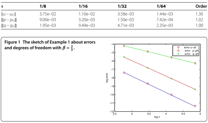
The numerical results for Example 1 are presented in Table 1, Table 2 and Figure 1. Table 1 shows that the convergence rate foruis 1 under theL2_{-norm, which exactly obey}

the prediction of Theorem 4.1. The convergence rates forqandpare 1 +γ +β₂ under the respective norms, which are almost close to the prediction of Theorem 4.1.

(13)

Table 1 Numerical results for Example 1 withτ= 2–12

β h 1/16 1/32 1/64 1/128 Order

1/4 u–uh 9.50e–03 4.78e–03 2.40e–03 1.20e–03 1.00

|||p–ph||| 3.33e–03 9.62e–04 2.81e–04 8.20e–05 1.78

|||q–qh||| 4.44e–03 1.43e–03 4.62e–04 1.50e–04 1.60

1/2 u–uh 9.48e–03 4.77e–03 2.39e–03 1.20e–03 1.00

|||p–ph||| 1.43e–03 3.94e–04 1.07e–04 2.79e–05 1.92

|||q–qh||| 3.90e–03 1.15e–03 3.45e–04 1.05e–04 1.73

2/3 u–uh 1.48e–02 7.53e–03 3.78e–03 1.89e–03 1.00

|||p–ph||| 6.15e–04 1.69e–04 4.54e–05 1.19e–05 1.94

|||q–qh||| 3.98e–03 1.09e–03 3.02e–04 8.37e–05 1.84

Table 2 Numerical results for Example 1 withh= 2–8_and_β₌2 3

τ 1/8 1/16 1/32 1/64 Order

u–uh 3.21e–03 1.25e–03 5.72e–04 2.83e–04 1.00

|||p–ph||| 1.23e–03 6.36e–04 3.21e–04 1.60e–04 1.00

|||q–qh||| 4.12e–03 2.01e–03 1.01e–03 5.11e–04 0.98

Table 3 Numerical results for Example 2 withτ= 2–10

β h 1/16 1/32 1/64 1/128 Order

1/4 u–uh 3.62e–02 1.91e–02 9.77e–03 4.95e–03 0.99

|||p–ph||| 6.51e–02 3.84e–02 2.28e–02 1.35e–02 0.75

|||q–qh||| 1.13e–02 7.26e–03 4.69e–03 3.04e–03 0.63

1/2 u–uh 3.62e–02 1.91e–02 9.77e–03 4.95e–03 0.99

|||p–ph||| 1.84e–02 9.04e–03 4.48e–03 2.23e–03 1.00

|||q–qh||| 1.03e–02 6.11e–03 3.62e–03 2.15e–03 0.75

2/3 u–uh 3.62e–02 1.91e–02 9.77e–03 4.95e–03 0.99

|||p–ph||| 6.86e–03 2.99e–03 1.31e–03 5.82e–04 1.15

|||q–qh||| 8.18e–03 4.59e–03 2.58e–03 1.46e–03 0.82

Table 4 Numerical results for Example 2 withh= 2–8andβ=2₃

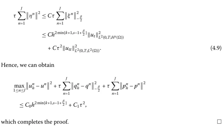
τ 1/8 1/16 1/32 1/64 Order

u–uh 3.75e–02 1.10e–02 3.58e–03 1.44e–03 1.30

|||p–ph||| 9.00e–03 3.20e–03 1.50e–03 7.42e–04 1.02

|||q–qh||| 1.95e–03 9.49e–03 4.71e–03 2.35e–03 1.00

Figure 1 The sketch of Example 1 about errors and degrees of freedom withβ=2₃.

Example 2 LetK = 1,θ = 1₂,T= 1. The analytic and smooth solution is prescribed to

beu(x) =x(1 –x)et _∈_H1+γ₍_{), and the source term} _f ₌_x_{(1 –}_x₎_et₊_et_(–xβ–1+(1–x)β–1 2(β) + xβ_+(1–_x₎β

(1+β) )∈H

(14)

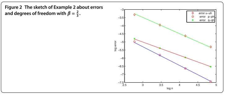
Figure 2 The sketch of Example 2 about errors and degrees of freedom withβ=2₃.

The numerical results are presented in Table 3, Table 4 and Figure 2.

Table 3 shows that the convergence rate foruis 1 under theL2-norm, which exactly obey the prediction of Theorem 4.1. The convergence rates forqandpareγ +β₂ under the respective norms, which are almost close to the prediction of Theorem 4.1.

Table 4 tests that the convergence rate in time. The numerical results show that the convergence rate foru,p,qin time is 1 which is consistent with the theoretical prediction by Theorem 4.1.

6 Concluding remarks

In this work, we establish the saddle-point variational formulation for a two-sided time-dependent fractional diﬀusion problem overH1₍₎_×_H–2β₍₎×_L2₍_{) and develop its}

fully discrete expanded mixed finite element procedure, which approximates optimally the unknown functionu, its derivativeqand the fractional fluxp. We find that the advantages of the mixed procedure at least are: (1) it can preserve the locally conservative property and can describe realistic fractional diffusive processes; (2) it is easily implemented since the standard finite element spaces are used.

Acknowledgements

This work is supported by NSF of China under Grants 11471196, 20142RB01849 and by NSF of Shandong province under Grant ZR2016JL004.

Competing interests

The authors declare that they have no competing interests.

Authors’ contributions

All authors contributed equally to this work. All authors read and approved the ﬁnal manuscript.

Publisher’s Note

Springer Nature remains neutral with regard to jurisdictional claims in published maps and institutional aﬃliations.

Received: 16 October 2017 Accepted: 7 January 2018

References

1. Mainardi, F: Fractional calculus. In: Carpinteri, A, Mainardi, F (eds.) Fractals and Fractional Calculus in Continuum Mechanics. Springer, New York (1997)

2. Shlesinger, MF, West, BJ, Klafter, J: Lévy dynamics of enhanced diﬀusion: application to turbulence. Phys. Rev. Lett.

58(11), 1100-1103 (1987)

3. Zaslavsky, GM, Stevens, D, Weitzner, H: Self-similar transport in incomplete chaos. Phys. Rev. E48(3), 1683-1694 (1993) 4. Sun, H, Hao, X, Zhang, Y, Beleanu, D: Relaxation and diﬀusion models with non-singular kernels. Phys. A, Stat. Mech.

Appl.468, 590-596 (2017)

(15)

6. Caputo, M, Fabrizio, M: A new deﬁnition of fractional derivative without singular kernel. Prog. Fract. Diﬀer. Appl.1, 73-85 (2015)

7. Singh, J, Kumar, D, Baleanu, D: On the analysis of chemical kinetics system pertaining to a fractional derivative with Mittag-Leﬄer type kernel. Chaos27(2017). https://doi.org/10.2298/TSCI170129096K

8. Kumar, D, Singh, J, Baleanu, D: Modiﬁed Kawahara equation within a fractional derivative with non-singular kernel. Therm. Sci. (2017). https://doi.org/10.1063/1.4995032

9. Kumar, D, Singh, J, Baleanu, D: A new fractional model for convective straight ﬁns with temperature-dependent thermal conductivity. Therm. Sci. (2017). https://doi.org/10.2298/TSCI170129096K

10. Beleanu, D, Jajarmi, A, Asad, J, Blaszczyk, T: The motion of a bead sliding on a wire in fractional sense. Acta Phys. Pol. A

131(6), 1561-1564 (2017)

11. Cui, M: Compact finite difference method for the fractional diffusion equation. J. Comput. Phys.228, 7792-7804 (2009)

12. Meerschaert, MM, Scheﬄer, HP, Tadjeran, C: Finite diﬀerence methods for two dimensional fractional dispersion equation. J. Comput. Phys.211, 249-261 (2006)

13. Li, C, Zeng, F, Liu, F: Spectral approximations to the fractional integral and derivative. Fract. Calc. Appl. Anal.15, 383-406 (2012)

14. Wang, H, Basu, TS: A fast finite difference method for two-dimensional space-fractional diffusion equations. SIAM J. Sci. Comput.34, 2444-2458 (2012)

15. Liu, Q, Liu, F, Turner, I, Anh, V: Finite element approximation for the modiﬁed anomalous subdiﬀusion process. Appl. Math. Model.35, 4103-4116 (2011)

16. Zhang, H, Liu, F, Anh, V: Garlerkin ﬁnite element approximations of symmetric space fractional partial diﬀerential equations. Appl. Math. Comput.217, 2534-2545 (2010)

17. Kumar, D, Singh, J, Baleanu, D: A new numerical algorithm for fractional Fitzhugh-Nagumo equation arising in transmission of nerve impulses. Nonlinear Dyn. (2017). https://doi.org/10.1007/s11071-017-3870-x

18. Kumar, D, Agarwal, RP, Singh, J: A modiﬁed numerical scheme and convergence analysis for fractional model of Lienard’s equation. J. Comput. Appl. Math. (2017). https://doi.org/10.1016/j.cam.2017.03.011

19. Hajipour, M, Jajarmi, A, Baleanu, D: An efficient non-standard finite difference scheme for a class of fractional chaotic systems. J. Comput. Nonlinear Dyn.13(2) (2017). https://doi.org/10.1115/1.4038444

20. Wu, G, Baleanu, D, Deng, Z, Zeng, S: Lattice fractional diﬀusion equation in terms of a Riesz-Caputo diﬀerence. Physica A438, 335-339 (2015)

21. Wu, G, Baleanu, D, Xie, H: Riesz Riemann-Liouville diﬀerence on discrete domains. Chaos26, 084308 (2016) 22. Ervin, VJ, Heuer, N, Roop, JP: Numerical approximation of a time dependent, nonlinear, space-fractional diﬀusion

equation. SIAM J. Numer. Anal.45, 572-591 (2007)

23. Ervin, VJ, Roop, JP: Variational formulation for the stationary fractional advection dispersion equation. Numer. Methods Partial Diﬀer. Equ.22, 558-576 (2005)

24. Ervin, VJ, Roop, JP: Variational solution of fractional advection dispersion equations on bounded domains inRd_.

Numer. Methods Partial Diﬀer. Equ.23, 256-281 (2007)

25. Deng, W, Hesthaven, JS: Discontinuous Galerkin methods for fractional diﬀusion equations. Math. Model. Anal.47(6), 1845-1864 (2013)

26. Li, Y, Chen, H: A mixed-type Galerkin variational formulation and fast algorithms for variable-coeﬃcient fractional diﬀusion equations. Math. Methods Appl. Sci.40(4), 5016-5034 (2017)

27. Jia, L, Chen, H: Mixed-type Galerkin variational priciple and numerical simulation for a generalized nonlocal elastic model. J. Sci. Comput.71(2), 660-681 (2017)

28. Raviart, PA, Thomas, JM: A mixed ﬁnite element methods for 2nd order elliptic problems. In: Mathmatical Aspects of the Finite Element Method. Lecture Notes in Maths., vol. 606, pp. 292-315. Springer, Berlin (1977)

29. Liu, Y, Du, Y, Li, H, Li, J, He, S: A two-grid mixed ﬁnite element method for a nonlinear fourth-order reaction-diﬀusion problem with time-fractional derivative. Comput. Math. Appl.70, 2474-2492 (2015)

30. Liu, Y, Fang, Z, Li, H, He, S: A mixed ﬁnite element method for a time-fractional fourth-order partial diﬀerential equation. Appl. Math. Comput.243, 703-717 (2014)

31. Wang, H, Yang, D, Zhu, S: A Petrov-Galerkin finite element method for variable-coefficient fractional diffusion equations. Comput. Methods Appl. Mech. Eng.290, 45-56 (2015)

32. Yang, S, Chen, H: Least-squared mixed variational formulation based on space decomposition for a kind of variable-coeﬃcient fractional diﬀusion problems. Manuscript

33. Oldham, KB, Spanier, J: The Fractional Calculus. Academic Press, New York (1974) 34. Podlubny, I: Fractional Diﬀerential Equations. Academic Press, New York (1999)

35. Samko, S, Kilbas, A, Marichev, O: Fractional Integrals and Derivatives: Theory and Applications. Gordon & Breach, London (1993)

36. Chen, H, Wang, H: Numerical simulation for conservative fractional diﬀusion equations by an expanded mixed formulation. J. Comput. Appl. Math.296, 480-498 (2016)

37. Brézzi, F, Douglas, J Jr., Fortin, M, Marini, L: Two families of mixed ﬁnite element for second-order elliptic problems. Numer. Math.47, 217-235 (1985)

38. Brézzi, F, Fortin, M: Mixed and Hybrid Finite Element Methods. Springer, Berlin (2011)

39. Chen, Z: Expanded mixed ﬁnite element methods for linear second-order elliptic equation. Math. Model. Anal.4, 479-499 (1998)