* Corresponding author: [email protected]
Mechanical behaviour modelling under dynamic conditions:
Application to structural and high strength steels
Pierre Simon1,2,*, Yaël Demarty1, and Alexis Rusinek2
1French-German research institute of Saint-Louis, 5 rue du general Cassagnou, 68300 Saint-Louis, France
2Laboratory of Microstructure Studies and Mechanics of Materials, UMR-CNRS 7239, Lorraine University, 7 rue Félix Savart, BP
15082, 57073 Metz Cedex 03, France
This work is in the framework of a PhD partially funded by the Direction General de l’Armement.
Abstract. Current needs in the design and optimization of complex ballistic protection structures lead to
the development of more and more accurate numerical modelling for high impact velocity. The aim of developing such a tool is to be able to predict the protection performance of structures using few experiments. Considering only numerical approach, most important issue to have a reliable simulation is to focus on material behaviour description in term of constitutive relation and failure model for high strain rates, large field of temperatures and complex stress states. In this context, the study deals with the behaviour of two steels including a high strength steel and a structural steel. For this application, the materials can undergo both quasi-static and dynamic loading. Thus the strain rate range studied is varying from 10-3 to more than 103 s-1. Although the high strength steels do not exhibit high strain rate sensitivity,
the temperature increases during dynamic loading is inducing thermal softening. Thus, temperature sensitivity is defined up to 500 K under quasi-static and dynamic conditions. Then, experiments are used to define the parameters of several constitutive relations like the Johnson-Cook model or the Rusinek Klepaczko model.
1 Introduction
The development of protective systems against ballistic impacts usually requires the use of several materials leading to complex structures. The design and optimization of such multi-layered structures is made possible through the use of numerical simulations. In fact, the number of parameters to consider (thickness, position of the materials, type of materials, etc.) is too significant to perform a parametric study using expensive and time consuming experimental campaigns.
Nevertheless, during experiment real mechanical material behaviour can be directly observed whereas in numerical model constitutive relations are used to describe it. Therefore, reliability of these relations is essential to obtain valid results. These material models usually represent the equivalent plastic stress of a material as a function of equivalent plastic strain, strain rate and temperature. Many relations have been developed through last decades, and are still under consideration. One can distinguish two main types of constitutive relations. The first ones are phenomenological, as they do not take into account any physical phenomenon and are only based on experimental observation. These relations have the main advantage of a low number of parameters. Nevertheless, their validity is most of time reduce at a small range of
condition. A well-known and widely implemented example of phenomenological model used for metals is the Johnson-Cook constitutive model [1]. The second category is semi-physical constitutive relations. Although these models are more complicate to handle because of their higher number of parameters, they allow a better representation of material behaviour and an extended range of validity, as they take into account physical consideration.
This study focuses on the dynamic mechanical behaviour of two distinct steels. The first one is a structural steel, while the second-one is a high strength steel which could be used as an armour steel. In a first part of this paper, the sensitivities to strain rates and temperature are studied. For this purpose, quasi-static and Hopkinson bar experiments were conducted. Positive and negative (only in dynamic regime) temperatures have been applied. The second part deals with the material modelling. Different constitutive models are presented and the identification of their related parameters is detailed. The third part shows a comparative study of the different models with the experimental results.
In order to determine the hardening, the strain rate and temperature sensitivities, compression tests have been performed. The studied range of strain rate is varying from 10-3 s-1 to more than 103 s-1. Regarding the
temperature, experiments allowed to observe material behaviour up to 473 K in both quasi-static and dynamic cases. Experiments at low temperature (down to 173 K) were also carried out in dynamic regime, using liquid nitrogen with addition of ethanol to adjust the temperature. Experiments at low strain rate from 10-3 to
10-1 s-1 have been performed using a quasi-static press,
while higher strain rates have been reached using split Hopkinson pressure bar technique.
2.1 Experiments at various strain rate
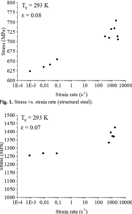
The stress value for each strain rate and assuming a strain level is represented, Fig. 1 and Fig. 2, for each steels. A strain value below 0.1 was chosen to reduce the adiabatic heating effect on the stress value. In both cases, the stress increases non-linearly with the strain rate.
1E-4 1E-3 0,01 0,1 1 10 100 1000 10000 600
625 650 675 700 725 750 775
800 T
0 = 293 K ε = 0.08
St
re
ss (
M
Pa
)
Strain rate (s-1)
Fig. 1. Stress vs. strain rate (structural steel).
1E-4 1E-3 0,01 0,1 1 10 100 1000 10000 1000
1050 1100 1150 1200 1250 1300 1350 1400 1450 1500 T
0 = 293 K ε = 0.07
St
re
ss
(M
Pa
)
Strain rate (s-1)
Fig. 2. Stress vs. strain rate (high strength steel).
2.2 Experiments at various temperature
Regarding experiments at high temperatures, each sample and the end of the bars have been heated for 30 minutes before the test to have a homogeneous
temperature distribution in the specimen [2]. The stress values for each temperature and a strain level imposed are reportedFig. 3 and Fig. 4. The stress decreases as the temperature increase. As for the strain rate sensitivity, the structural steel presents higher temperature sensitivity in comparison with the high strength steel.
3 Constitutive models
In this part, models are compared with experiments reported previously. It allows observing if the models are able to describe the material behaviour.
3.1 Johnson-Cook constitutive model
150 200 250 300 350 400 450 500 500
550 600 650 700 750 800 850 900 950
1000 ε ~ 1400 to 1700/s
ε = 0.001/s ε = 0.08
St
res
s (
M
Pa)
Temperature (K) Fig. 3. Stress vs. Temperature (structural steel).
150 200 250 300 350 400 450 500 1000
1050 1100 1150 1200 1250 1300 1350 1400 1450 1500 1550
1600 ε ~ 1000/s
ε = 0.001/s
St
re
ss (
M
Pa
)
Temperature (K) Fig. 4. Stress vs. Temperature (high strength steel).
The Johnson-Cook model is a phenomenological model describing material behaviour through the Eq. (1) [1].
, , = + 1 + log 1 − ∗ (1)
where A, B, C, n and m are the model parameters and T*
is the homologous temperature. The parameters A, B and
n are determined by fitting stress vs. plastic strain curve at defined conditions , T0. Effects of the strain rate and
third terms, by taking stress value at a fixed level of plastic strain. Therefore, the parameters are easy to identify although this model presents some limits. Firstly, as strain rate and temperature effects are separated, no coupling effect can be taken into account. Moreover, no modification of the hardening as well as no temperature below the reference temperature (in this work, room temperature) can be represented by this model.
3.2 Rusinek-Klepaczko constitutive model
This semi-physical model [3] is based on the theory of dislocations and decomposes the stress in an internal stress and an effective stress, Eq. (2).
, , = , , + ∗ , (2)
Where E(T) and E0 represent the Young Modulus as
function of the temperature and its value at 0 K. Although this value can vary, the evolution of Young modulus of steels [4] is assumed to be low enough (between 173 and 473 K) to be neglected. The internal stress is expressed by the Eq. (3):
, , = , + , (3)
Where B and n are strain rate and temperature hardening coefficients. ε0 is the strain level defining the yield
stress. Eq. (4) and (5) show how are defined B and n:
, = log
(4)
, = 〈1 − log 〉 (5)
Finally, the effective stress is given by the Eq. (6).
∗
, = ∗〈1 − log 〉∗ (6)
Where B0, ν, n0, D2, σ0*, D1 and m* are the model
parameters, and are its limits of validity. The
operator 〈〉 = if > 0 and 〈〉 = 0 otherwise. The internal stress represents the evolution of the dislocation density (creation and annihilation) which is affected by strain (hardening) but also by strain rate and temperature [5]. At the opposite, the effective stress describes an instantaneous effect. From a physical point of view, it represents the difficulty of a dislocation to overcome an obstacle. This additional stress tends to vanish as the temperature increases and increases when the strain rate increases [4]. Therefore, the model neglects this stress at low strain rates for room and higher temperatures.
The first step of the identification of the parameters allows defining D1, such as the effective stress is equal
to zero at low strain rate (10-3 s-1 in the present case) and
293 K as suggested by the Eq. (7).
= log .
(7)
Assuming that the effective stress is equal to zero at low strain rate, it allows to determine a first approximation of 0.001,293 and 0.001,293. As the effective stress corresponds to an instantaneous effect and the internal stress to a history effect, the next step of the identification assumes that at a given strain level (below 0.1 to assume isothermal conditions), the evolution of stress is mainly due to the thermal activation process. Then the Eq. (8) allows to determine the values of σ0* and m.
∗, = , , − , 0.001,293 (8)
Once the effective stress is defined, values of
, and , for different sets of conditions can
be identified. Finally, Eq. (4) and (5) are used to determine B0, ν, n0 and D2.
4 Evaluation and comparison of the
constitutive models
4.1 Johnson-Cook model
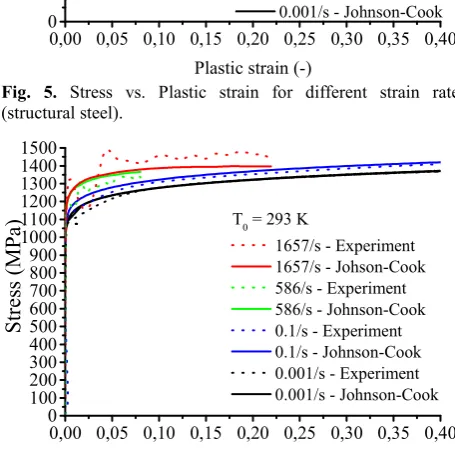
A Comparison between experiments and the Johnson-Cook model is shown in Fig. 5 and Fig. 6, for both steels. As the strain rate varies during dynamic experiments, an average value is used.
Hardening is well represented by the model in quasi-static conditions, meaning that the first terms of Eq (1) provides a good description of the materials behaviour in these conditions. Nevertheless, in the dynamic regime, one can observe that the model does not fit experimental data and has a trend to deviate for the highest strain rate. The Johnson-Cook model assumes a linear sensitivity of the stress as a function of the logarithm of the strain rates. As shown in Fig. 1 and Fig. 2, strain rate sensitivity is not linear for these steels, but increase for dynamic cases. This explains why this model does not give a good description of materials behaviour for dynamic cases. This problem is especially relevant for the structural steel, as the strain sensitivity is higher than for the high strength steel.
conditions and in dynamic conditions. Therefore, this model does not permit to describe temperature dependency of the mechanical behaviour of the structural steel over the whole range of the studied strain rates.
0,00 0,05 0,10 0,15 0,20 0,25 0,30 0,35 0,40 0 100 200 300 400 500 600 700 800 900 1000
St
ress
(M
Pa)
Plastic strain (-)
T0 = 293 K
1719/s - Experiment 1719/s - Johson-Cook 429/s - Experiment 429/s - Johnson-Cook 0.1/s - Experiment 0.1/s - Johnson-Cook 0.001/s - Experiment 0.001/s - Johnson-Cook
Fig. 5. Stress vs. Plastic strain for different strain rate (structural steel).
0,00 0,05 0,10 0,15 0,20 0,25 0,30 0,35 0,40 0 100 200 300 400 500 600 700 800 900 1000 1100 1200 1300 1400 1500
St
res
s (
M
Pa)
Plastic strain (-)
T0 = 293 K
1657/s - Experiment 1657/s - Johson-Cook 586/s - Experiment 586/s - Johnson-Cook 0.1/s - Experiment 0.1/s - Johnson-Cook 0.001/s - Experiment 0.001/s - Johnson-Cook
Fig. 6. Stress vs. Plastic strain for different strain rate (high strength steel).
0,00 0,05 0,10 0,15 0,20 0,25 0,30 0,35 0,40 0 100 200 300 400 500 600 700 800 900 1000 St res s ( M Pa)
Plastic strain (-)
ε = 1719/s
293 K - Experiment 293 K - Johnson-Cook 348 K - Experiment 348 K - Johnson-Cook 398 K - Experiment 398 K - Johnson-Cook
Fig. 7. Stress vs. plastic strain for different temperature (structural steel).
0,00 0,02 0,04 0,06 0,08 0,10 0,12 0,14 0 100 200 300 400 500 600 700 800 900 1000 1100 1200 1300 1400 1500 St re ss (M Pa )
Plastic strain (-) ε ~ 1100/s
323 K - Experiment 323 K - Johnson-Cook 373 K - Experiment 373 K - Johnson-Cook 473 K - Experiment 473 K - Johnson-Cook
Fig. 8. Stress vs. plastic strain for different temperature (high strength steel).
4.2 Rusinek-Klepaczko model
A comparison between experiments at different strain rates and the model is shown on the Fig. 9 and Fig. 10. Regarding the structural steel, this model allows to represent non-linear sensitivity, with a lower sensitivity in quasi-static than in dynamic. Although, the sensitivity in quasi-static is too low to represent experiment performed at 0.1/s, this model provides good representation of the experiments in most of the case studied. Regarding the high strength steel, this model provides a better representation than the Johnson-Cook model.
0,00 0,05 0,10 0,15 0,20 0,25 0,30 0,35 0,40 0 100 200 300 400 500 600 700 800 900 1000 St re ss ( M Pa )
Plastic strain (-)
T0 = 293K
1719/s - Experiment 1719/s - Rusinek-Klepaczko 429/s - Experiment 429/s - Rusinek-Klepaczko 0.1/s - Experiment 0.1/s - Rusinek-Klepaczko 0.001/s - Experiment 0.001/s - Rusinek-Klepaczko
0,00 0,05 0,10 0,15 0,20 0,25 0,30 0,35 0,40 0
100 200 300 400 500 600 700 800 900 1000 1100 1200 1300 1400 1500
St
ress
(M
Pa)
Plastic strain (-) T0 = 293 K
1657/s - Experiment 1657/s - Rusinek-Klepaczko 586/s - Experiment 586/s - Rusinek-Klepaczko 0.1/s - Experiment 0.1/s - Rusinek-Klepaczko 0.001/s - Experiment 0.001/s - Rusinek-Klepaczko
Fig. 10. Stress vs. plastic strain for different strain rate (high strength steel).
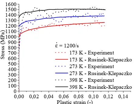
Regarding experiment at various temperatures, this model provides, for both steels, a good description. The stress is slightly over-estimated for the structural steel at 173 K, but is well represented at other temperatures. Regarding the high strength steel, all temperatures of the range studied, including the case at 173 K are well represented by this model.
0,00 0,05 0,10 0,15 0,20 0,25 0,30 0,35 0,40 0
100 200 300 400 500 600 700 800 900 1000 1100 1200
St
re
ss (
M
Pa
)
Plastic strain (-) ε = 1719/s
173 K - Experiment 173 K - Rusinek-Klepaczko 273 K - Experiment 273 K - Rusinek-Klepaczko 398 K - Experiment 398 K - Rusinek-Klepaczko
Fig. 11. Stress vs. plastic strain for different temperature (structural steel).
0,00 0,02 0,04 0,06 0,08 0,10 0,12 0,14 0
100 200 300 400 500 600 700 800 900 1000 1100 1200 1300 1400 1500 1600
St
re
ss (
M
Pa
)
Plastic strain (-) ε = 1200/s
173 K - Experiment 173 K - Rusinek-Klepaczko 273 K - Experiment 273 K - Rusinek-Klepaczko 398 K - Experiment 398 K - Rusinek-Klepaczko
Fig. 12. Stress vs. plastic strain for different temperature (high strength steel).
5 Conclusion
The mechanical behaviours of a structural steel and a high strength steel has been studied, with experiments performed at various strain rates varying from 10-3 s-1 to
103 s-1 and various temperature going from 173 K to 473
K. The parameters of the constitutive relations were identified and the results were compared to experiments. The first one is the Johnson-Cook constitutive model. This model allows a good description of temperature sensitivity for both steel, but only for temperature above its reference temperature (293 K in this work). Furthermore, it assumes a linear strain rate sensitivity, which is not the case of the materials studied. Therefore, a good representation of the dynamic and quasi-static cases cannot be obtained with this model. The second model studied is the Rusinek-Klepaczko constitutive model. At the opposite of the previous model, it is a semi-physical model and allows a better representation of strain rate sensitivity for both materials. Moreover, temperature sensitivity is also well represented, including for experiments performed at temperatures below 293 K.
References
1. G.R. Johnson, W.H. Cook, (1983)
2. A. Rusinek, R. Bernier, R. Matadi Boubimba, M. Klosak, T. Jankowiak, G. Voyiadjis, Polymer Testing, 65, 1-9, (2018)
4. A. Rusinek, J.R. Klepaczko, Int. J. of Plasticity, 17, 87-115, (2000)
4. J. Klepaczko, A. Rusinek, J.A. Rodriguez-Martinez, Pecherski. R.B., A. Arias, Mech. of Mat., 41, 599-621 (2009)