Gravity wave spectra morphology in the Arctic and non-Arctic lower atmosphere

(1)

Scholarship@Western

Electronic Thesis and Dissertation Repository

9-25-2014 12:00 AM

Gravity wave spectra morphology in the Arctic and non-Arctic

lower atmosphere

Melanie C. Wright

The University of Western Ontario

Supervisor

Wayne K. Hocking

The University of Western Ontario Graduate Program in Physics

A thesis submitted in partial fulfillment of the requirements for the degree in Master of Science © Melanie C. Wright 2014

Follow this and additional works at: https://ir.lib.uwo.ca/etd

Part of the Fluid Dynamics Commons, and the Other Physics Commons

Recommended Citation Recommended Citation

Wright, Melanie C., "Gravity wave spectra morphology in the Arctic and non-Arctic lower atmosphere" (2014). Electronic Thesis and Dissertation Repository. 2520.

https://ir.lib.uwo.ca/etd/2520

This Dissertation/Thesis is brought to you for free and open access by Scholarship@Western. It has been accepted for inclusion in Electronic Thesis and Dissertation Repository by an authorized administrator of

(2)

(Monograph)

by

Melanie Wright

Faculty of Science

Department of Physics and Astronomy

Submitted in partial fulfillment of the requirements for the degree of

Master of Science in Physics

The School of Graduate and Postdoctoral Studies The University of Western Ontario

London, Ontario, Canada August, 2014

(3)

ii

Abstract

The spectral analysis of data from three VHF radars (one high-Arctic and two mid-latitude)

show general support for the universal spectrum theory for gravity waves in the lower

atmosphere (altitudes of 2.0-11.0 km), provided that the impact of the off-vertical beam and

noise are taken into consideration. This analysis also reveals that local gravity wave

generation is of secondary, but still significant, importance for determining the spectra.

A total of eight spectral methods were considered and scrutinized for the purposes of

determining gravity wave spectra from VHF radar data. A definition for the “best” method

was given and examined. The method selected as the “best” for the analysis presented was a

date-compensated discrete Fourier transform with a Hamming window.

Keywords

(4)

iii

Acknowledgments

I would like to thank the family and friends who have been most supportive of me

completing my masters and during my time at Western, specifically (in no specific order):

Gram Char and Grandpa Gary, Neil Bhatt, Jason Kirkness, John and Betty Kirkness, Emma

Cookson, Amanda DiCarlo, Mat Abado, Rob Weryk, and the lovely people at Dance Steps

(specifically Donna Bayley and Krista Conti).

I want to thank Emily McCullough for the use of her Matlab plotting function

(imagescnanEmily), which has been included in Appendix B. I would also like to thank

CANDAC for partial funding, including: Bob Sica, Pierre Fogal, Jim Drummond, and Ashley

Kilgour. I would also like to thank the ladies in the Physics and Astronomy Department

office (Clara, Jodi, Jackie, Lisa, Nelia, Loveleen, and Donna) who have been extremely

helpful, as well as my advisory committee: Bob Sica and John de Bruyn.

Above all else, I would like to extend my deepest gratitude to my supervisor, Wayne

Hocking, who has supported and pushed me the whole way through. I couldn’t have asked

(5)

iv

List of Figures

Figure 2.1 ... 4

Figure 2.2 ... 9

Figure 3.1 ... 12

Figure 3.2 ... 13

Figure 3.3 ... 14

Figure 3.4 ... 17

Figure 3.5 ... 20

Figure 3.6 ... 21

Figure 3.7 ... 22

Figure 3.8 ... 22

Figure 4.1 ... 25

Figure 4.2 ... 27

Figure 4.3 ... 30

Figure 4.4 ... 31

Figure 4.5 ... 32

Figure 4.6 ... 33

Figure 4.7 ... 34

Figure 4.8 ... 36

(10)

ix

Figure 4.10 ... 39

Figure 5.1 ... 41

Figure 5.2 ... 43

Figure 5.3 ... 44

Figure 5.4 ... 45

Figure 5.5 ... 46

Figure 5.6 ... 47

Figure 5.7 ... 47

Figure 5.8 ... 48

Figure 5.9 ... 48

Figure 5.10 ... 50

Figure 5.11 ... 51

Figure 5.12 ... 52

Figure 5.13 ... 53

Figure 5.14 ... 54

Figure 5.15 ... 55

Figure 5.16 ... 56

Figure 6.1 ... 69

Figure 6.2 ... 70

(11)

x

Figure 7.1 ... 78

(12)

Chapter 1

1 Introduction

In 1960, Hines suggested internal gravity waves (or buoyancy waves) as a major

contributor to upper atmosphere motions, carrying energy and momentum large distances

through the atmosphere. The literature fixated on singular waves until, in 1982,

VanZandt proposed a “universal spectrum”—a shape to the intensity of gravity waves

versus their wavenumber that is independent of geographic location, meteorological

conditions, altitude, and time—based on the oceanographic work of Garrett and Munk

(1972, 1975). The literature absorbed the concept of universality: many (e.g. Medvedev

and Klassen 2000) produced power spectral density forms based on theories such as

Weinstock’s nonlinear wave diffusion, Hines’ Doppler shifted theory, and the

inconsistent linear instability theory (Hines 1991). Focus then shifted towards deviations

from the spectrum (e.g. Eckermann 1995), which leaves us thinking, “How ‘universal’ is the universal spectrum anyway?”

I investigate the form of the gravity wave spectra at different geographic locations

(Negrocreek, ON and Eureka, NU) and altitudes (selected altitudes between 1-14 km) in

different seasons. My analysis using Ferraz-Mello’s (1981) data-compensated discrete

Fourier transform with a Hamming window reveals that “universality” is not a far-fetched

idea; however, local gravity wave generation also affects the gravity wave spectra.

This thesis is comprised of seven chapters. Chapter 2 reviews the gravity wave

literature and provides motivation for this work. The necessary prerequisite background

on radars is given in Chapter 3. Chapter 4 outlines the mathematical background to the

analysis methods including reasoning for applying windows and selecting various

analysis techniques. Chapter 5 applies the methods described in Chapter 4 to determine

the “best” method of computing atmospheric gravity wave spectra. The results are

presented and interpreted in Chapter 6. Chapter 7 concludes this thesis and outlines

(13)

Chapter 2

2 Gravity waves

Gravity waves (also known as buoyancy waves), named for the restoring force

responsible for the wave motion, are perturbations in the atmosphere (density, pressure,

velocity, and temperature) with typical horizontal wavelengths of a few to hundreds of

kilometres, vertical wavelengths of approximately , and periods of five

minutes to many hours. In general, these waves can propagate along the interface of two

mediums (such as on the surface of a lake or ocean, where they are called surface gravity

waves) or through a medium (such as through the ocean or atmosphere, where they are

called internal gravity waves), provided that the density decreases with increasing height.

This thesis specifically examines the geographical and temporal variation of the spectrum

of atmospheric internal gravity waves, which will be referred to as “gravity waves”.

2.1 Why gravity waves

Atmospheric gravity waves have a large impact on aircraft and weather. Early interest in

mountain lee waves (a particular type of gravity wave, generated by flow over

mountains) originated from sailplane pilots, who used the waves to soar to record

altitudes (Gossard and Hooke 1975). Waves can transport energy faster than mean flow

transport. In particular, gravity waves carry energy away from the source (a mountain

range, thunderstorm, etc.) and distribute it throughout the atmosphere, produce

phenomena such as turbulence in the night time atmospheric boundary layer or clear air

turbulence (Nappo 2002), which can be hazardous to aircraft (Gossard and Hooke 1975).

In addition to playing a major role in upper atmosphere dynamics (Hines 1960),

gravity waves can slow—and even reverse—mean wind speeds throughout the

atmosphere, including in the troposphere (e.g., Lindzen 1981, Holton 1983). A better

(14)

2.2 Gravity wave overview

While both surface and internal gravity waves propagate in a similar manner, it may be

easier for the reader to conceptualize gravity waves using surface gravity waves, for

example, on the surface of a lake. Consider a small packet of water displaced vertically

above the lake’s surface. The mass of water above the mean level causes the surface of

the water to fall. When the water surface reaches equilibrium, it still has a downwards

momentum and continues to fall. The surrounding water applies a restoring force to the

water surface, causing it to slow the downwards motion, eventually stop, and then return

towards the equilibrium position. The surface overshoots equilibrium again, causing it to

be displaced above the water surface again, hence establishing an oscillation. This

motion propagates along the surface.

Internal gravity waves propagate in the same manner, however, the atmosphere

must satisfy a second condition (in addition to decreasing density with height); having a

specific lapse rate. A lapse rate is the rate at which air temperature decreases with

increasing altitude. For internal gravity waves to propagate through the atmosphere, the

lapse rate of the air packet as it moves must be steeper than the lapse rate of the

background atmosphere. As air rises, it expands and becomes less dense. After rising,

the air packet needs to be denser than the surrounding air to oscillate. If it isn’t, the air

packet will continue rising, instead of oscillating, and internal gravity waves cannot

occur. Where the lapse rates are such that internal gravity waves can propagate, the

atmosphere is called “stable”. Otherwise, the atmosphere is called “unstable”.

2.3 Causes of gravity waves

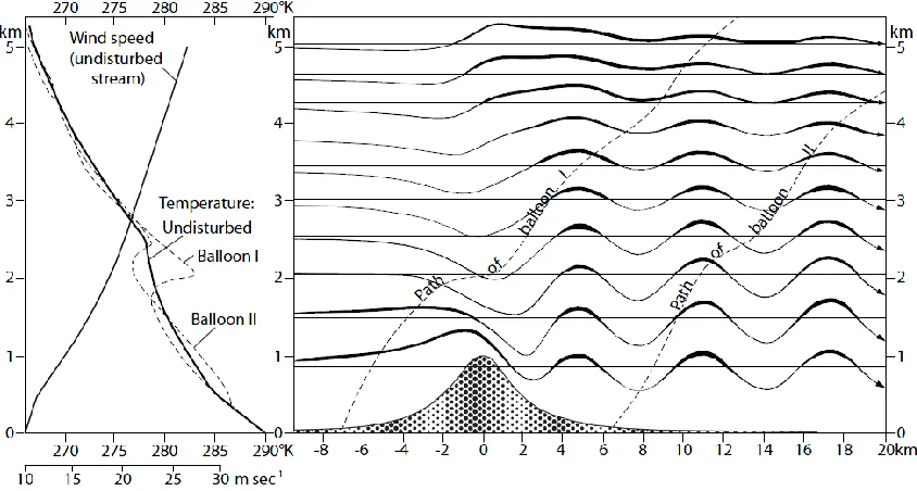
One well accepted source of gravity waves is airflow over terrain, such as mountains and

hills (Gossard and Hooke 1975). Airflow over mountains causes the initial perturbation

necessary to create waves, as demonstrated in Figure 2.1. These waves are also known as

“mountain lee waves”. In a steady state, these waves are stationary with respect to the

terrain, but propagate with respect to the mean airflow. In a time-dependent state, airflow

(15)

Figure 2.1: An example of mean wind flow over a mountain causing lee-waves and the accompanying mean wind and temperature structure. From Hocking (in prep.), adapted from Röttger (2000) (who adapted it from Scorer (1997)).

occasions Hines suggested (e.g. Hines 1991) that this may cause waves in the upper

atmosphere.

Other potential sources of gravity waves are: squall lines and frontal systems,

velocity jets, large explosions (Nappo 2002), turbulence, penetrative convection,

wave-wave interactions, geostrophic adjustment, shear instability, Ekman-layer instability, and

wave generation by boundary-layer turbulence (Gossard and Hooke 1975).

2.4 A brief history of the understanding of gravity waves

In 1960, Hines explored the theory of gravity waves as a major contributor to upper

atmosphere motions. He used linear perturbation theory, which assumes that the wave

amplitudes (the perturbations in pressure, temperature, etc.) are sufficiently small, such

that all variables dependent on nonlinear combinations of wave amplitudes are negligible.

(16)

though he still treated the nonlinear pressure terms as negligible, since the pressure

fluctuations are relatively small.

The literature focused on singular gravity wave sightings and measurements until

1982, when Van Zandt introduced the idea of a “universal spectrum” of gravity waves,

based on the oceanic work of Garrett and Munk (1972, 1975). The universal spectrum

quantifies the spectral “tail” (lower wavelengths) as a power law and claims the shape of

the tail is roughly invariant with meteorological conditions, latitude and longitude, time,

and, to some extent, altitude.

In 1991, Hines developed a Doppler spread theory for gravity waves. In general,

literature focus shifted to this concept of universality, with many research groups

developing similar models to describe the universality. Focus then shifted to deviations

from universality.

2.5 Mathematical Background

The mathematics of gravity waves starts with the standard fluid dynamics equations (a

version of Newton’s second law, the first law of thermodynamics combined with the

speed of sound in air, conservation of mass, and heat diffusion, respectively), viz.:

⃗⃗

⃗⃗ ⃗

⃗⃗

⃗

(2.1)

(2.2)

⃗⃗ ⃗

(2.3)

(2.4)

where represents differentiation following the motion, ⃗ is the velocity, is the

density, ⃗⃗ is the Earth’s angular rotation rate, is the acceleration due to gravity (and is

(17)

differential operator, is the potential temperature, is the heat diffusion coefficient,

and is the kinematic viscosity coefficient.

For gravity waves, solutions are assumed to be of the form:

( ⃗ ) (2.5)

where can be any one of the velocity components, the pressure, the density, or

temperature, and may be complex. ⃗ is the wavenumber vector and refers to

the ground-based angular frequency of the wave. These forms are substituted into the

standard fluid dynamics equations above, keeping only first-order perturbation terms in

an attempt to linearize the equations for gravity wave analysis. If the effects of viscosity

are ignored, a mean wind of zero is assumed (for simplicity), and the wave propagates in

the — plane (with being vertical), then the standard fluid dynamics equations (i.e.

Equations 2.1 through 2.4) simplify to five equations; three momentum equations:

̂ ̂ ̂

(2.6)

̂ ̂

(2.7)

̂ ̂ ( ̂

̂_̅

)

(2.8)

a form of the first law of thermodynamics:

̂

_̅̅̅̂ (2.9)

and a continuity equation:

̂ ̂

̂

(2.10)

where a hat (e.g., ̂) denotes a perturbation value, √ , is the Coriolis parameter

(18)

of sound at the height of the wave. The complex velocity perturbation is ⃗ ̂ ̂ ̂ .

The ⃗ -vector is , where it is assumed that the wave propagates in the — plane

for simplicity. The complex vertical wavenumber, , is (complex to indicate

that the wave is oscillating and the amplitude increases exponentially with increasing

height), where ̅ . ̅ is the scale height given by:

̅

̅ (2.11)

The Brunt-Vaisala frequency, , is the natural oscillation frequency of a displaced air

parcel in the atmosphere (below 100 km altitude, values are typically 5-10 minutes) and

satisfies:

̅ ̅

̅ ̅ ̅

(2.12)

where , is the gas constant for air, is the specific heat of air at constant

pressure, and is potential temperature.

Solutions to these equations are various waves that satisfy two particular relations:

the dispersion relation and polarization relations. The dispersion relation relates the wave

frequencies and wavenumbers. It also restricts wave frequencies to the range between the

Brunt-Vaisala frequency and the “inertial frequency”, the lower frequency limit set by the

Coriolis parameter. The polarization relations relate wave-velocity amplitudes to the

temperature, density, and pressure amplitudes. Both the dispersion and polarization

relations can differ slightly, depending on the terms ignored/retained in the linearized

approximations to the equations of motion.

For the approximated equations of motion, the dispersion relation is:

(19)

A simpler form of the approximation, called the Boussinesq approximation, is:

(2.14)

for a wide range of frequencies larger than and smaller than , this dispersion

relations can be approximated by:

(2.15)

The polarization relation is approximated by the following equations:

̂

_̅

̂

(2.16)

̂

(2.17)

̂

̅

̂

̅

̂

̅ ̂

̅

̂

(2.18)

̂ ̅

̂

̅ (2.19)

̂ ̂ ̅ ̅

(2.20)

where ̂ is the vertical displacement, and ̅ is the “intrinsic phase speed” of the wave, or the wave phase speed with respect to the mean wind at the height of the

wave. Equations 2.16 and 2.17 are exact for the Boussinesq approximation and

Equations 2.18, 2.19, and 2.20 are only valid for .

More precise relations can be developed; however, these approximations are useful since

they are simple, yet are still fairly accurate over a wide range of frequencies. Unlike the

(20)

2.6 The spectral tail

While the theory of gravity wave spectra in the atmosphere and oceans is very similar,

VanZandt (1982) summarized three key differences: (1) Doppler shifting by mean flows

is more important in the atmosphere, (2) nonlinear wave interactions occur over shorter

timescales, and (3) the atmospheric buoyancy frequency is roughly independent of

height, whereas it decreases exponentially with depth in the ocean.

In the atmosphere, the slope of the tail is roughly invariant with altitude and

flattens off at lower frequencies (see the sample tail in Figure 2.2). At higher altitudes,

the tail is longer (i.e. flattens off at a lower frequency). Van Zandt (1982) claimed this

(21)

was the result of saturation of particular frequencies and left the physical cause for

separate identification.

Hodges (1967, 1969) introduced linear perturbation theory to model gravity

waves, which assumes that the wave amplitudes are small enough such that the nonlinear

terms are negligible. When gravity waves propagate upwards in the atmosphere, the

wave amplitudes grow exponentially (due to exponentially decreasing density). Some

authors (e.g. Lindzen 1981, 1984) used linear instability theory to account for the form

and intensity of the tail; at a critical height, the linear approximation breaks down and

above this height, nonlinearities cause saturation. Hines (1991) reworked the linear

instability formulation and found inconsistencies. Hines (1991) created a Doppler shifted

theory which accounts for the intensity and the form of the spectral tail, claiming that

linear instability theory may account for the length of the tail.

Another potential cause of gravity wave saturation is shedding. As waves

increase in altitude, their amplitude increases as well. At a critical height (dependent on

the frequency of the wave), the wave grows too big and any energy that would normally

cause an increase in amplitude dissipates as turbulence instead.

Extending Weinstock’s (1976) nonlinear wave diffusion theory and Hines’ (1991)

Doppler spreading theory, Medvedev and Klaassen (2000) explained saturation by

turbulence induced in waves that exceeded the convective instability thresholds. They

parameterized the power spectral density, , as:

(2.21)

where is roughly a constant (which slowly varies with and the mean wind), is the

Brunt-Vaisala frequency, and is vertical wave number. Throughout the literature,

values of range from to (see Medvedev & Klassen, 2000), with values typically

being (e.g. Smith et al. 1987). Other literature even has dependent on seasons. This

model gives reasonable magnitudes for acceleration of mean flow and some observations

(22)

for use in parameterization schemes because it has a clear physical interpretation.

However, it has some disadvantages too; the theory only works for near monochromatic

waves, it requires the gravity wave amplitudes to be nearly constant at and above the

breaking level, and, when using this model, the vertical wave drag profiles and enhanced

(23)

Chapter 3

3 Radars

3.1 The antennas

The radars used to gather data for this thesis do not use a large dish for transmitting and

receiving the signal, but rather use a large array of smaller antennas that work together as

one coherent unit. This is called a "phased array" and its beam can be steered without

actually tilting the ground upon which the antennas rest. The specific radars for this

study are comprised of 128 antennas (called Yagi antennas). In the arrays used, each

antenna acts as both a transmitter and receiver. The antennas have three horizontal bars;

from the top down, they are: the director, the driven element, and the reflector.

(24)

3.2 How they work

The transmitter, under the control of the computer, sends an electronic pulse to the

antenna array and each antenna transmits the pulse as an electromagnetic wave. Since

there are many antennas transmitting the same pulse simultaneously (an exception, i.e.

beam steering, is discussed below), the transmitted pulse appears as a plane wave

propagating vertically upward from the array, as demonstrated in Figure 3.2. Each of the

planar waves is an interference pattern caused by the individual antenna wavelets. The

waves reflect off targets (or more specifically, gradients in refractive index) in the

atmosphere. Some of the reflected wave propagates back towards the antenna array.

The reflected wave induces a current in the driven element (the middle horizontal

bar). The director and reflector play the role of narrowing the radar beam, and so in some

senses "concentrating" the signal. After going through hardware processing, the voltage

is digitized at a rate corresponding to (in our case) intervals.

3.3 Beam steering

The 3D interference pattern created by the antennas is called the beam pattern. The beam

pattern represents the "pattern of sensitivity" of the radar, with targets in the regions of

highest sensitivity being most strongly detected; i.e. the direction of the beam pattern

defines where the radar is “looking”. The beam pattern is the diffraction pattern of the

antennas and, therefore, depends on the layout of the antennas and their orientation with

(25)

smaller beams (called sidelobes), which point in different directions than the main beam.

Since the sidelobes are smaller (i.e. lower power), most of the atmospheric detections

occur through the main lobe. The effect of sidelobes is discussed below.

In the case described above, the main beam points perpendicular to the plane of

the radar (normally vertical). To steer the beam (to “look” in other directions), a time

delay is applied between nearby antennas transmitting the same pulse, as seen in Figure

3.3.

Figure 3.3: A schematic describing how the radar beam is steered through the sky. Rather than transmitting the pulse simultaneously, the left-most antenna started transmitting, followed by the second from the left, the third from the left, and then the rightmost antenna. Typically delays are a small fraction of one wave-period; in our case typically or so.

3.4 Detection difficulties

3.4.1 Detection through sidelobes

Since the main beam is large in strength (so it has more power) in comparison to the

sidelobes, it is assumed that targets detected are located within the main beam. However,

a strong reflector (e.g. a plane, a building, etc.) in a side lobe will have the same effect as

a weaker reflector in the main beam.

Once the radar is built (i.e. the position of the antennas is set), there is not much

(26)

called "interferometry" can be used to obtain better directional information, but this

requires extra antennas and is not needed for our particular studies.

3.4.2 Non-atmospheric objects

It’s a bird! It’s a plane! It’s not an atmospheric target. The targets in the atmosphere are

weak reflectors (small density changes) and typically move relatively slowly (most

velocities are less than ). When something with strong reflectance is in the radar

volume or an object moves unusually fast through the radar volume, it has a stronger

influence on the data than the atmospheric targets. However, their distinct nature often

allows them to be recognized and ignored.

The power returned to the antenna array depends on the square of the potential

refractive index gradient. The refractive index in the lower atmosphere is:

_(3.1)

where is the pressure in millibars, is the temperature in Kelvin, and is the partial

water vapour pressure in millibars. Sometimes this equation also contains a plasma term,

which is unnecessary in the region of interest for this study. The gradient is given by

(Tatarski 1961, with updated constants from Larsen and Röttger 1982):

[

] [

]

(3.2)

where is the temperaure in degrees celsius, is the adiabatic lapse rate, and is the specific humidity. The power received by the radar, , is

proportional to the square of the refractive index gradient, viz.:

(3.3)

Therefore, larger refractive index gradients, such as those between the atmosphere and a

bird or plane, return more power to the radar than smaller refractive index gradients, such

(27)

Often, highly reflective, non-atmospheric objects (e.g. birds, airplanes) do not

stay in the radar volume for very long, perhaps a few tens of seconds. Such targets can

be removed in two ways: (1) recognizing the characteristic signature of the entity and

removing it from the data-stream or (2) simply ignoring the entire data set. Typically

calculation of a wind measurement requires of data, so if such a group is too

severely contaminated, the entire data set is ignored.

Another type of non-atmospheric target that gets detected is ground clutter (e.g.

mountains and buildings). Reflections from ground clutter enter the radar beam through

the sidelobes and are seen as having zero velocity. Various tricks can be used to remove

these contaminants, but they are only partly successful. In this thesis, we primarily use

data collected using an off-vertical beam, since the horizontal movement of the air

(generally) produces non-zero radial velocities and ground clutter (which occurs at )

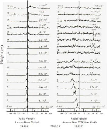
can be notched out. Vertical beams are harder to use because the vertical winds are often

close to zero and merge in with the ground-clutter, making separation of the different

spectral sources more difficult, as shown in Figure 3.4.

3.4.3 Poor low altitude range data: impedance mismatch

If the impedance of the antenna and the cables are not exactly the same, then when the

transmitted pulse passes from the coaxial cable to the antenna, some of the signal is

reflected. The reflected signal propagates back along the coaxial cable and is reflected at

the transmitter end since it is not expecting to receive a signal of that strength (the

receiver is disconnected when the voltage is over a particular threshold). The reflected

signal propagates back to the antenna where some is reflected again and some is

transmitted. This oscillation leads to a ringing after the pulse has been transmitted.

Sometimes this ringing interferes with receiving reflections from the pulse scattered from

atmospheric targets. This often results in unreliable data for the lower end of the radar’s

range ( for the radars used in this thesis), so conclusions here-in are primarily

(28)

(29)

3.4.4 Poor high altitude range data: low power

If the scatterers are particularly weak, the reflected wave may go undetected by the radar.

This is particularly true for the higher altitudes of the radar’s range ( for the

radars used in this thesis) for a variety of reasons.

The power transmitted from the radar diminishes in strength proportionally to the

range squared. Upon reflection, the power of the reflected wave also diminishes

proportionally to the range squared, so the power received by the radar diminishes as the

range to the power . This is partially compensated for by the fact that the radar

volume (where the atmospheric targets are detected) increases proportionally to the range

squared. This still results in a net loss of returned power. Specifically, the received

power is inversely proportional to the square of the range—scatterers at altitude

return times less signal than scatterers at altitude.

The properties of the atmosphere also come into play. Air density decreases

exponentially with altitude—air density at is times less than at the ground—

resulting in a loss of scattering capability. Furthermore, the scattering cross-section also

depends on water vapour content to some extent. Water vapour densities are

considerably less at altitude. All these factors combine to mean that above

(typically) altitude, the signal is too weak for our radars to detect.

3.4.5 Range determination and range-aliasing

The radar sends out a pulse, then “listens” for a response. The distance from the radar to a

target (the range of the target) is determined from the expression:

(3.4)

where is the speed of light in air (the speed at which the pulse propagates) and is the

time between the radar pulse-transmission and pulse reception. In practice, there will be

multiple targets and so multiple received pulses at different lags. The factor of comes

from the fact that the observed time is twice the time the wave took to get from the radar

(30)

denote range as opposed to an (implying height) since if the beam is pointing in a

direction other than vertical, range and height are different.

The detection process assumes that everything detected is a reflection from a

target due to the last pulse that was transmitted. This is not always true; sometimes a

pulse from a very distant target may return to the radar after a subsequent pulse was

transmitted, resulting in range aliasing (incorrectly calculating the range) for detections

farther away than:

(3.5)

where is the time between successive radar pulses. Since the radar is not designed to

detect reflections above , the returned pulses from beyond are generally weak;

however, a strong reflection (e.g. meteor) at a higher altitude may still reflect the pulse

such that it is detected by the radar.

For an example, consider a radar that transmits pulses at an interval allowing it to

see up to away. If a meteor at range reflected the pulse, the radar would

interpret the meteor reflection as happening at range (a reflection from the most

recently transmitted pulse) as opposed to (a reflection from the fourth last pulse,

which is the true pulse of origin for the scattered pulse).

3.5 Why radar? (As opposed to other methods)

Consistent, short time interval data are needed for this study. Radar is the only method

that gathers atmospheric measurements of this nature.

In-situ measurements, such as rockets and weather balloons, can yield very

detailed data. With in-situ measurements, the experimenter has no control over what

section of atmosphere it samples and the time between successive launches (

hours) is too long for this study.

Other ground-based measurements (mainly lidar) can provide successive, highly

(31)

nights. For mid-latitude sites, the lidar would be unoperational every day during sunlit

hours, which would not be ideal. For Arctic sites, the lidar would be unoperational for

the entire summer (as the sun does not set). These gaps in data collection are not well

suited for this study. Recent developments have allowed newer lidars to work in the

daytime as well, but they are still restricted by fog and clouds and—for the present—are

primarily useful below or so in height (Stiller et al. 2012).

3.6 Our sites

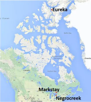
This thesis uses three Canadian radar sites; Eureka, Negrocreek, and Markstay (as shown

in Figure 3.5). All three sites consist of 128 Yagi antennas and operate somewhere in the

band 46-51 MHz, with specific frequencies being different at each radar.

(32)

3.6.1 Eureka, Nunavut

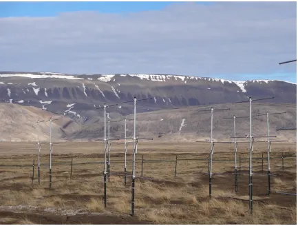
Eureka, Nunavut (pictured below) is a high-Arctic site at GPS coordinates 80.00 N, 85.80

W. The radar at Eureka is surrounded by Arctic tundra. The radar operates at 51.0 MHz

and has been operational since 2007.

Figure 3.6: A panoramic view of the radar station at Eureka, NU with Blacktop mountain in the distance. The computer and transmitter are located inside the blue-green building to the right.

3.6.2 Negrocreek, Ontario

Negrocreek (pictured in Figure 3.7) is located in southern Ontario at GPS coordinates

44.36 N, 80.86 W near the town of Owen Sound, near the Great Lakes. The land at

Negrocreek is swampy and surrounded by trees. The radar operates at 48.92 MHz and

has been operational since 2008.

3.6.3 Markstay, Ontario

Markstay (picture in Figure 3.8) is also located in Ontario, north of Negrocreek at GPS

coordinates 46.54N, 80.54 W, a short distance from Sudbury. The area surrounding

Markstay is mostly forest and Canadian shield. The radar operates at 45.47 MHz and has

(33)

Figure 3.7: Part of the radar station at Negrocreek, ON.

(34)

Chapter 4

4 Spectral analysis methods

A repetitive function or signal can be represented as a superposition of simple sine and

cosine waves, sometimes referred to as harmonics. However, in a more developed

theory, even non-periodic functions can be represented in this way, provided that an

infinite number of frequencies are available. The Fourier transform of a function

determines which frequencies, and the amplitude of each frequency that the harmonics

require, in order to sum to the original function. For a continuous function in time, ,

the Fourier transform has many equivalent definitions; however, this thesis will use the

definition:

∫

(4.1)

for all real and , where represents time (in seconds) and represents frequency (in

hertz).

The power spectrum (relative power of each harmonic vs. frequency) is often used

to analyse the harmonics of a signal. The power spectrum intensity is given by:

‖ ‖

(4.2)

The remainder of this chapter discusses issues arising from using the Fourier transform

with our specific data (finite, discrete, and non-uniformly spaced data), and our solutions

to those problems (windowing functions and the date-compensated discrete Fourier

transform).

4.1 Finite Data

In practice, the measured signal is not infinite in extent, and the Fourier transform is

usefully redefined as:

(35)

where represents the signal length and the hat on the signifies the finite data signal

(which, for this section, is continuous; discretizing the signal causes other effects, which

are discussed later). For the purposes of this thesis, ̂ is one component of the

radar-derived wind velocity. In terms of the ideal, infinite signal, the finite signal is:

̂

(4.4)

where is a boxcar window function:

{

(4.5)

so that:

̂ ∫

(4.6)

From this perspective, it is evident that the finite nature of the data intrinsically applies a

window function. This has deleterious effects in the frequency domain, causing a

broadening of spectral frequencies and “frequency leakage”.

Multiplying the signal by the window function applies the window to the signal.

In the frequency domain, this is equivalent to convolving the signal’s Fourier transform and the window function’s Fourier transform. To see the full effects of a window,

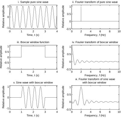
consider a pure sine wave. The Fourier transform of a pure sine wave is a delta function

at the wave’s frequency, as shown in Figure 4.1 (ii). The Fourier transform of a boxcar

window function is a sinc function, as shown in Figure 4.1 (iv). The Fourier transform of

a pure sine wave, after applying a boxcar window to it, is a sinc function (the boxcar’s Fourier transform) centred at the sine wave’s frequency, as shown in Figure 4.1 (vi).

Note that the boxcar Fourier transform has a main lobe centred at zero with smaller

“sidelobes” on either side. While a wider main lobe broadens spectral peaks, the

sidelobes spread spectral frequencies to higher and lower frequencies.

However, a boxcar is only one type of window. Sometimes, spectral clarity

(36)

that such a process would further deteriorate the spectrum, but advantages ensue due to

reduction of the sidelobes. Since using a windowing function is unavoidable, a variety of

window functions were examined.

Figure 4.1: A demonstration of how a multiplication in the time domain is equivalent to a convolution in the frequency domain. (i) A pure sine wave, (iii) a boxcar window function, and (v) the product of (i) and (iii). The plots in the right column are the corresponding Fourier transforms of the plots shown to their immediate left.

0 1 2 3 4

-1 0 1

i. Sample pure sine wave

Time, t (s)

R e la ti v e a m p lit u d e

0 2 4 6 8 10

-0.5 0 0.5 1

ii. Fourier transform of pure sine wave

Frequency, f (Hz)

0 1 2 3 4

-1 -0.5 0 0.5 1

iii. Boxcar window function

Time, t (s)

0 2 4 6 8 10

-0.5 0 0.5 1

iv. Fourier transform of boxcar window

Frequency, f (Hz)

0 1 2 3 4

-1 0 1

v. Sine wave with boxcar window

Time, t (s)

0 2 4 6 8 10

-0.5 0 0.5 1

vi. Fourier transform of sine wave with boxcar window

Frequency, f (Hz)

(37)

4.2 Windows

Creating the “best” window is a result of optimizing the main lobe width and relative

amplitude of the sidelobes. Since the data set is finite, there will always be sidelobes;

however, they can be suppressed at the expense of widening the main lobe (broadening

the main lobe is equivalent to smearing frequencies into neighbouring frequencies in the

frequency domain). Similarly, the main lobe can be narrowed at the expense of

increasing the sidelobes (potentially leading to frequency aliasing). Both large sidelobes

and a wide main lobe are detrimental to the spectra. Four windows are examined in this

thesis to determine the optimal window for the gravity wave spectra. The windows

examined here are: boxcar, boxcar with 10% cosine tapering, Hann (sometimes called

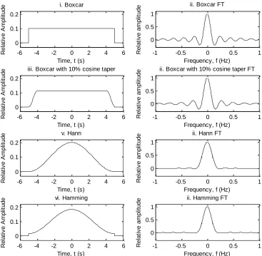
Hanning), and Hamming. The windows and their Fourier transforms are displayed in

Figure 4.2. The normalization and Fourier transform of each window are displayed

step-by-step in the Appendix.

4.2.1 Boxcar window

The boxcar window (Figure 4.2(i)) for a signal length of is:

{ | |

(4.7)

The boxcar window may appear to be ideal because it gives each data point equal

weighting. However, the sudden start and stop of the data causes detrimental ringing in

the frequency domain.

4.2.2 Boxcar with 10% cosine taper window

The boxcar with 10% cosine taper (Figure 4.2 (iii)) for a signal length of is:

{

(

)

| |

(

)

(38)

This window gives 80% of the data equal weighting and uses the outside 20% (10% at

the beginning and 10% at the end) to smooth the ringing effect of the sudden start and

stop.

Figure 4.2: The left column contains representations of all the windows applied to data sets in this thesis. While the windows in plots (i), (iii), (v), and (vii) span 10 seconds in this sample, when applied to the data in this thesis, they span the same length of time as the data (typically a month). The plots in the right column are the Fourier transform of the plots shown to their immediate left.

-6 -4 -2 0 2 4 6

0 0.1 0.2

Time, t (s)

R e la ti v e A m p lit u d

e i. Boxcar

-6 -4 -2 0 2 4 6

0 0.1 0.2

Time, t (s)

e iii. Boxcar with 10% cosine taper

-6 -4 -2 0 2 4 6

0 0.1 0.2

Time, t (s)

e v. Hann

-6 -4 -2 0 2 4 6

0 0.1 0.2

Time, t (s)

e vi. Hamming

-1 -0.5 0 0.5 1

0 0.5 1

Frequency, f (Hz)

R e la ti v e a m p lit u d

e ii. Boxcar FT

-1 -0.5 0 0.5 1

0 0.5 1

Frequency, f (Hz)

e ii. Boxcar with 10% cosine taper FT

-1 -0.5 0 0.5 1

0 0.5 1

Frequency, f (Hz)

e ii. Hann FT

-1 -0.5 0 0.5 1

0 0.5 1

Frequency, f (Hz)

(39)

4.2.3 Hann window

The Hann window, named for Julius von Hann, (Figure 4.2(v)) is the discrete window

function:

(

)

(4.9)

for { | }, where is the sample size. For the purposes of this section (to

demonstrate the effects of a windowing function rather than the effects of discretization

of data), the Hann window is treated as the continuous function:

{

(

) | |

(4.10)

where is the signal length and the window has been shifted so that its centre is at .

The Hann window widens the main lobe to minimize the amplitude of all side lobes.

4.2.4 Hamming window

The Hamming window, named for Richard W. Hamming, (Figure 4.2(vii)) is the discrete

window function:

(

)

(4.11)

for { | }, where is the sample size. For the purposes of this section, the

Hamming window is treated as the continuous function:

{ (

(

)) | |

(4.12)

where is the signal length, is the normalization constant , and the window has

been shifted so that its centre is at . Unlike the other windows in this thesis, the

(40)

. While the Hann window aims to reduce the effect of all sidelobes, the Hamming

window aims to reduce the first side lobe as much as possible.

4.3 Discrete Data

A second issue arises when trying to use the Fourier transform; the Fourier transform is

defined for a continuous signal and the radar collects discrete data. Discretizing the data

is equivalent to multiplying the continuous signal (i.e. the north component of the wind

velocity in our case) by a sampling function; specifically a series of Dirac delta functions

evenly spaced at an interval of . The sampling function is:

∑

(4.13)

The Fourier transform of the sampling function is another sampling function:

∑

(4.14)

where the spacing in the temporal and frequency domains are related by:

(4.15)

Recalling that a multiplication in the temporal domain is a convolution in the frequency

domain, multiplying the signal by a sampling window leads to repetition of the signal’s

Fourier transform in the frequency domain, as Figure 4.3 demonstrates.

In order to determine a frequency, it must be sampled at least twice per cycle. If a

frequency is sampled less frequently, it appears as a wave of lower frequency. For a

visual example, see Figure 4.4. Any wave of frequency , which is above half the

sampling frequency (termed the Nyquist frequency), appears as the lower frequency:

(4.16)

where is the Nyquist frequency ( ). This implies that all frequencies larger

(41)

4.5 to Figure 4.7. Figure 4.5 is a sample spectrum. If the data were discretized at a rate

of 20 Hz, the resulting calculated spectrum would be given by Figure 4.6. Figure 4.7

shows how the sample spectrum and resulting spectrum are related. Non-equally

sampled data may produce harmonics beyond the Nyguist frequency. This would add to

the noise level at all frequencies and the harmonics would be aliased to the wrong

frequency.

Figure 4.3: The Fourier transform of a pure sine wave with a frequency of 10 Hz, sampled at a frequency of 30 Hz. The Nyquist frequency (denoted as Nyq in the figure) is half the sampling frequency (15 Hz). Beyond the Nyquist frequency, the spectrum repeats itself as described in the text.

0 10 Nyq 25 2*Nyq 40 3*Nyq 55 4*Nyq

0 0.2 0.4 0.6 0.8 1

Frequency, f (Hz)

R

e

la

ti

ve

a

mp

lit

u

d

(42)

Figure 4.4: The solid line shows a pure sine wave with frequency 1/10 Hz. The black circles represent the sine wave if it were sampled at a rate of 1/12 Hz. However, the black dots also correspond to a sine wave of frequency 1/60 Hz ( ), shown by the dashed line. If a 1/10 Hz sine wave was sampled at 1/12 Hz, the Fourier transform would mistake the original sine wave as a 1/60 Hz sine wave. This leads to frequency aliasing when data are digitized too slowly.

0

20

40

60

80

100 -1

-0.5

0

0.5

1 Time, t (s)

R

e

la

ti

ve

a

mp

lit

u

d

(43)

Figure 4.5: A sample spectrum created to demonstrate the effects of sampling at an insufficiently high frequency. The spectral peaks occur at frequencies: , , , and . See Figure 4.6 for the final result of sampling at a frequency of . See Figure 4.7 to see why that is the case.

0 5 10 15 20 25 30 35 40

0 0.1 0.2 0.3 0.4 0.5 0.6 0.7 0.8 0.9 1

Frequency, f (Hz)

R

e

la

ti

ve

a

mp

lit

u

d

e

(44)

Figure 4.6: The resulting calculated spectrum when the data set that was created in Figure 4.5 is sampled at a frequency of 20 Hz. Notice that the four peaks present in the sample spectrum ( , , , and in Figure 4.5) appear at , , , and , respectively. Figure 4.7 shows the relation between the sample spectra and this calculated spectra.

0 2 4 6 8 10

0 0.2 0.4 0.6 0.8 1 1.2 1.4

Frequency, f (Hz)

R

e

la

ti

ve

a

mp

lit

u

d

e

(45)

Figure 4.7: (i) The portion of the original spectrum in Figure 4.5 between 0 Hz and the Nyquist frequency (10 Hz). (ii) The portion of the original spectrum in Figure 4.5 between the Nyquist frequency and twice the Nyquist frequency. (iii) The portion of the original spectrum in Figure 4.5 between twice the Nyquist frequency and thrice the Nyquist frequency. (iv) The portion of the original spectrum in Figure 4.5 between thrice the Nyquist frequency and four times the Nyquist frequency. (v) The spectrum resulting from sampling the data for Figure 4.5 at 20 Hz and (as a result) the sum of plots (i) through (iv) as they are lined up. Since the data in this example are sampled at 20 Hz, frequencies in plots ii, iii, and iv are mapped onto the range [ ]. This can be seen in more detail in Figure 4.6.

0 Nyq 0 0.5 1 R e la ti ve a m p li tu d

e i. Portion of spectra between 0 and Nyq

Nyq 2*Nyq 0 0.5 1 R e la ti ve a m p li tu d

e ii. Portion of spectra between Nyq and 2*Nyq

2*Nyq 3*Nyq 0 0.5 1 R e la ti ve a m p li tu d

e iii. Portion of spectra between 2*Nyq and 3*Nyq

3*Nyq 4*Nyq 0 0.5 1 R e la ti ve a m p li tu d

e iv. Portion of spectra between 3*Nyq and 4*Nyq

0 1 2 3 4 5 6 7 8 9 10

0 0.5 1 R e la ti ve a m p li tu d

e v. Resulting calculated spectrum

(46)

4.4 Fast Fourier transform

To summarize thus far, the Fourier transform of a set of data from the radar is:

̃ ∫ ̃

(4.17)

where ̃ is the radar data given by:

̃

(4.18)

where is the continuous atmospheric phenomenon, is the window function, and

is the sampling function. A simpler, more computer friendly method of computing

Equation 4.17 is to implement the definition of the discrete Fourier transform (DFT)

instead of the continuous version above. The DFT is defined as:

̂

∑

̂

(4.19)

for discrete points, where , and ̂ is the discrete windowed radar data (i.e.

).

4.5 Non-Uniformly Spaced Data

The radar data are non-uniformly spaced in time for a variety of reasons. On long time

scales, interruptions to the radar’s operation (due to, for example, power interruption or

equipment failure) require on-site technical intervention from London, ON. This is not

always feasible on a short timescale, leading to missing periods of data. While

Negrocreek and Markstay are approximately a 2-3 and 6-8 hour drive one way

respectively, Eureka is an expensive, fly-in only service run. Figure 4.8 depicts when the

radar sites were operational.

Even when the radars are operational, the data sampling rate is inconsistent, as

shown in Figure 4.9Error! Reference source not found.. In some cases, the data were

gathered for previous studies, which may have been collected at different sampling rates.

(47)

If a wind velocity differs from the nearest neighbouring measurements by more than

(user-definable), it is discarded as it is unlikely to be atmospheric data in the

Figure 4.8: Black represents the radar site being non-operational. Where the radar sites are operational (white), uniformly spaced data may still be unavailable. The number on the ordinate is the year. For ease of reading, the radar site names (Eureka, Negrocreek, and Markstay) are shortened to just the first initial (E, N, and M respectively).

Jan Feb Mar Apr May Jun Jul Aug Sep Oct Nov Dec

E

2007

N E

2008

N E

2009

M N E

2010

M N E

2011

M N E

2012

M N E

2013

M N E

(48)

expected radar volume (recall range aliasing, non-atmospheric scatterers, and detection

through sidelobes). For some atmospheric conditions, the radar is unable to measure

within the extremes of its range (e.g. not enough power, pulse saturation), resulting in

missing data for low (roughly 1.0-3.0 km altitude) and high (roughly 12.0-14.0 km

altitude) ends of the radar’s range.

While there are numerous methods of coping with non-uniformly spaced data

(e.g., Lomb-Scargle (Lomb 1976, Scargle 1982), MUSIC (Marple 1987,etc.), this thesis

examines two solutions: (1) using averaging of bins and interpolating when necessary to

use the fast Fourier transform and (2) using the date-compensated discrete Fourier

transform.

(49)

4.6 Bin averaging and interpolation

In an attempt to reduce the amount of interpolating necessary due to short-term (on the

order of minutes to a few hours) non-uniform data, the radar data are averaged in bins of

15 minutes. When there are empty bins, the gaps are interpolated. The interpolation is

linear between the data points immediately before and after the empty bins, with random

noise added. The same standard deviation is used for the interpolated data as exists in the

bins near the missing one(s) (5 points before and 5 points after). Missing gaps of data are

not interpolated if the gap spans six hours or longer. As such, one month may have

multiple “strands” of data to compute the spectra and spectral slope. In this case, the

longest data strand is selected as representative for the month. The Fourier transform is

then calculated using Matlab’s built in FFT function.

Matlab’s built-in FFT uses a combination of algorithms, including: the

Cooley-Tukey algorithm (Cooley & Cooley-Tukey 1965), a variation of Cooley-Cooley-Tukey (Oppenheim

1989), a prime factor algorithm (Oppenheim 1989), a split-radix algorithm (Duhamel &

Vetterli 1990), and Rader’s algorithm (Rader 1968). For more information on the details

of solving the DFT, see Matlab’s help page on FFT.

4.7 Date-compensated discrete Fourier transform

The second method this thesis uses to cope with non-uniformly spaced data is the

date-compensated discrete Fourier transform (DCDFT), as proposed by Ferraz-Mello (1981),

which computes a power spectral density estimate for discrete, unequally time-spaced

data. For a particular frequency, , this method involves fitting the following three

curves to the data (after they are orthonormalized in a Gram-Schmidt fashion and the

mean of the data is removed), as presented in Ferraz-Mello (1981):

(4.20)

(4.21)

(50)

This fit provides a power spectral density estimate to the data for frequency . To obtain

a power spectrum for this thesis, this process is repeated for frequencies evenly spaced

between where is number of data points in the signal. In the special case of

equally time-spaced data, the DCDFT simplifies to the discrete Fourier transform.

4.8 Spectral slope

Once the Fourier transform of the radial velocities is determined and converted into a

power spectrum, the slope is determined. All of the slopes are determined using a least

squares fit to the frequencies between 6 hours and 2 days (approximately

_{). The upper bound of the period range (i.e. 2 days) is the}

upper boundary to gravity wave periods. The lower bound (i.e. 6 hours) was chosen such

that it does not include the shallowing of the noise floor. A sample spectrum is shown in

Figure 4.10 with the green line showing the spectral slope for the section included in the

calculation.

(51)

Chapter 5

5 Spectral method selection

This thesis examines two different ways of determining the monthly spectra with four

different windows at three different radar sites. To save on computation, the different

methods are illustrated in detail for only one of the sites (Negrocreek, a mid-latitude site)

for one year, with some comparisons to a second site (Eureka, a high-latitude site). All

sites, and a wider coverage of years, are presented once the methodologies are optimized.

The year 2009 was selected as the comparison year since both Eureka and

Negrocreek were operational for the majority of that year. The “best” method of

determining spectra is chosen from this comparison and then used to compare all three

radar sites (Eureka, Negrocreek, and Markstay) over their operational periods (7, 6, and 4

years respectively).

5.1 Definition of “best”

Each of the monthly spectra for Negrocreek for each altitude and each window type was

examined visually and the “breakpoint” frequency was selected manually. The

breakpoint frequency separates the portion of the spectrum with an identifiable non-zero

slope—sometimes referred to as the “signal” portion—and from the noise floor. Figure

5.1 shows a sample spectra with the breakpoint indicated. The breakpoint value is used

to determine which method is “best”; the higher frequency the breakpoint, the more of

the spectra can be seen (i.e. is not hidden in noise). Figure 5.2 to Figure 5.5 compare the

breakpoint frequency between different windows and methods.

The plots depicting the breakpoint frequency as a function of altitude and month,

Figure 5.2 to Figure 5.5, show the difference in the breakpoint frequency between two

methods (i.e. FFT or DCDFT) with the same window. The methods being compared are

noted on the colour bar axis. The site and window that is being held constant is noted at

the top of the figures. Similarly, Figure 5.10 to Figure 5.16 show the difference in the

(52)

Figure 5.1: A typical monthly spectrum, indicating the breakpoint frequency. This spectrum is for Negrocreek, January 2009 using the DCDFT method with the Hamming window.

compared are noted on the colour bar axis (the boxcar with 10% cosine taper window is

shortened to “10% cos”). The site and method that is being held constant is noted at the

top of the figures. The colour indicates which of the method and window combinations

has a higher break point (i.e. lower noise floor and are preferred). A more intense colour

implies that one method/window combination has a higher breakpoint frequency than the

other. However, the most intense colours do not necessarily imply a large difference in

breakpoint frequency. For spectra that did not have a noise floor (i.e. the majority of the

spectra is noise), the breakpoint frequency was set to zero. Where this is the case for one

window (at a particular range gate in a specific month) and not the second, that

colour-coding at the appropriate altitude, month coordinate will appear as an intense colour

(53)

breakpoint frequency. White values imply that the spectra for both windows did not have

a noise floor. These plots demonstrate this definition of best.

There is a second criterion to the “best” as well. Atmospheric phenomena, such as

gravity waves and their spectra, are expected to be fairly continuous as a function of

altitude and time. Since the spectra used in this thesis are monthly averages, the spectra

are not necessarily expected to be continuous from month to month; however, they

should still be roughly continuous as a function of altitude. Spectral methods that yield

erratic spectral slopes as a function of altitude are probably not an accurate description of

the physical scenario. Therefore, the second criteria to being the “best” is that the slopes

are smooth functions with altitude.

5.2 The “best” method

Under the breakpoint definition of “best”, the fast Fourier transform (FFT) method

appears better than the date-compensated discrete Fourier transform (DCDFT) for all

windows.

While the FFT appears to be the better choice, the spectral slopes computed with

the FFT are more erratic than those computed with the DCDFT. Figure 5.6 to Figure 5.9

depict the spectral slopes using the FFT and DCDFT methods for a representative

window for both Negrocreek and Eureka in 2009. These plots depict the erratic

behaviour of the spectral slopes when analyzed with the FFT method. The apparent

better choice of breakpoint frequency for the FFT is possibly an artifact, as is described in

Chapter 6.

It is also possible that the FFT frequencies have been aliased, due to the

time-interval binning of data. More analysis on the spectral methods is needed to reveal if this

(54)

Figure 5.2: Comparisons between frequency break points at the junction between the signal and the noise floor for the DCDFT compared to the FFT for the boxcar window. In this case, 80 comparisons show a preference (i.e. a larger break point frequency) for the DCDFT while 241 show a preference for the FFT. Since this plot is overwhelmingly cyan, the FFT yields a lower noise barrier than the DCDFT.

Gravity wave spectra morphology in the Arctic and non-Arctic lower atmosphere

Scholarship@Western

Scholarship@Western

Gravity wave spectra morphology in the Arctic and non-Arctic

Gravity wave spectra morphology in the Arctic and non-Arctic

lower atmosphere

lower atmosphere

Abstract

Keywords

Acknowledgments

Table of Contents

List of Figures

Chapter 1

1

Introduction

Chapter 2

2

Gravity waves

2.1

Why gravity waves

2.2

Gravity wave overview

2.3

Causes of gravity waves

2.4

A brief history of the understanding of gravity waves

2.5

Mathematical Background

⃗⃗ ⃗

⃗⃗

⃗

⃗⃗ ⃗

̂ ̂ ̂

̂ ̂

̂ ̂ ( ̂

)

̂

̂ ̂

̂

̅

̂

̂

̂

̂

̂

̂

̂

̂

̅ ̂

̂

̂ ̂ ̅ ̅

2.6

The spectral tail

Chapter 3

3

Radars

3.1

The antennas

3.2

How they work

3.3

Beam steering

3.4

Detection difficulties

3.4.1

Detection through sidelobes

3.4.2

Non-atmospheric objects

[

] [

]

3.4.3

Poor low altitude range data: impedance mismatch

3.4.4

Poor high altitude range data: low power

3.4.5

Range determination and range-aliasing

3.5

Why radar? (As opposed to other methods)

3.6