SIMULATION AND PREDICTION OF PROCESS PARAMETERS IN CNC TURNING ON AISI 316L MATERIAL THROUGH REGRESSION HYBRID PSO ALGORITHM

258 | P a g e

SIMULATION AND PREDICTION OF PROCESS

PARAMETERS IN CNC TURNING ON AISI 316L

MATERIAL THROUGH REGRESSION HYBRID PSO

ALGORITHM

D.Ramalingam

, Dr.M.Saravanan

, R.Rinu Kaarthikeyen

1

Associate Professor, Nehru Institute of Technology, Kaliyapuram, Coimbatore-641105 (India)

2

Principal, SSM Institute of Engineering and Technology, Dindigul-624002 (India)

3

Research Associate Manager – Engineering, TCMPFL, Chennai-600051 (India)

ABSTRACT

Turning process is the most advantageous machining process and very commonly used by the manufacturing industries. AISI 316L steel material have the application in medical field as biomaterials, biomedical implants, biocompatible materials it requires the most desired surface quality. Obtaining the required surface quality is one of the major challenge and the prime responsibility in the manufacturing operations. Analyzing and optimizing the combination of the input machining parameters to achieve the desired surface finish is taken as the objective of this attempt with the Particle Swarm Optimisation technique in MATLAB programming. Referring to the convergence performance of the PSO the hybridization regression equations in the PSO and the regression computed values of parameters feed as input the further simulation carried out. The results are found to be more tuned in each phase of the simulation. The optimised parameter combinations for gorgeous surface finish are identified.

Key words: AISI 316L steel material, Turning, Regression, Particle Swarm Optimisation,

Hybridization, Minitab, MATLAB.

I. INTRODUCTION

Because of the superior corrosion resistance to inter granular corrosion, to most chemicals, salts, acids and high

creep strength at elevated temperatures AISI 316L steel material is preferred in the application in medical field

as biomaterials, biomedical implants, biocompatible materials, chemical processing, food processing,

photographic, pharmaceutical, textile finishing, marine exterior trim. As a special material, the surface finish

quality warrants high degree of importance in these applications. During manufacturing bringing the required

surface quality is the most common challenge because of the variables involving in the machining are having its

own impact on the outcome of the processing either individual or in combination. The most common primary

input machining parameters are machining speed, tool feed into the work material and the depth of cut in each

259 | P a g e

focused towards the analysis and optimisation of primary machining variables cutting speed, feed and depth of

cut on the resultant parameter surface roughness and laying a smooth path in turning operations on AISI 316L

material.

Abbreviations Used

S Cutting speed R-sq R - square statistical value

DOC Depth of cut R-sq (adj) R - square adjusted statistical value

Exp Experiment R-sq (pred) R - square predicted statistical value

F Feed rate Reg Regression

PSO Particle Swarm Optimization Ra Surface Roughness

II. RELATED LITERATURE

The significant importance of the surface roughness property is recognized by all researchers and manufacturers

as this characteristic has a direct impact on the serviceable attributes of any product. So as to achieve reasonable

surface quality with dimensional accuracy and precision, it is crucial to make use of the optimization

methodologies to achieve the objectives. Suresh et al. [1] have applied the Response Surface Method and

genetic algorithm in order to forecast the surface finish and optimized the progression parameters. Several

researchers made attempts to predict the surface quality in turning operation through applying neural network

techniques as well as statistical modeling. Mital and Mehta [2] have developed a modelling with statistical

approach in their research towards the surface roughness. M.A. El-Baradie [3] has coined surface roughness

modeling to predict the reasonable outcome while turning the grey cast iron material with the BHN value of

154. El-Sonbaty and Megahed [4] have applied the neural network technique in their investigation on turning

operations. Hasegawa et al. [5], Sahin Y and Motorcu [6,7], G. Petropoulos et al. [8], Grzesik and Wanat [9]

have made considerable amount of contributions through their investigations and devised surface modeling to

establish the required and desirable surface quality. Lin et al. [10] applied the Response Surface Methodology

to predict the surface roughness in their experiments. Gopal and Rao [11] also explained the application of

Response Surface Methodology in the surface quality prediction modelling through experimental investigation

in grinding operations. Singh and Kumar [13] employed the micro-genetic algorithm implementation to conduct

the optimization process in turning operations on EN-24 steel. Nikolaos et al. [12] have investigated in detail

about the surface roughness prediction in turning process on AISI 316L material. Agapiou [14] explained the

suitability of regression analyses applications to find the optimal levels and to analyze the effect of the drilling

parameters on surface finish. Oezel and Karpat [15] have reported that the surface roughness is primary results

of process parameters such as tool geometry and cutting conditions (such as feed rate, cutting speed, depth of

cut, etc.). Emad Ellbeltagi et al. [16] offered a paper on comparison among five evolutionary–based

optimization algorithms (GA, MA, PSO, ASO, and SFL). They concluded that, the PSO method was generally

found to perform better than other algorithms in terms of success rate and solution quality. Saravanan et al. [17]

applied the non-traditional techniques for cutting parameters optimization (GA, SAA, TS, MA, ACO and the

260 | P a g e

quality. Achala et al. [19] have investigated the turning process dynamics through the MATLAB software as a

platform. The principal purpose of this investigation is to study the influence of the input machining parameters

during turning operation on the average surface roughness of the machined surface. The examination and

forecasting of optimized parametric combination is recognized through the application of PSO algorithm

through MATLAB programming. A narrative approach of feeding the regression equation relationship as input

instead of random approach and the experimental output values are replaced with the regression values.

III. EXPERIMENTAL WORKS AND MATHEMATICAL MODELING

On the AISI 316L steel material which has the mechanical properties listed in the Table 3.1, turning experiment

has been conducted in the CNC lathe OKUMA Lb 10II model by Nokolaos [12] as the material is holding the

application in medical field as biomaterials, biomedical implants, biocompatible materials, chemical processing,

food processing, photographic, pharmaceutical, textile finishing, marine exterior trim. This material is preferred

because of the superior corrosion resistance to inter granular corrosion, to most chemicals, salts, and acids. Also

have high creep strength at elevated temperatures.

Table 3.1 Mechanical properties of AISI 316L material

Hardness, Rockwell B 79 HRB Elongation of break 50%

Tensile strength, ultimate 560 MPa Modulus of elasticity 193 GPa

Tensile strength, yield 290 MPa Poisson's ratio 0.29

The cutting tool material used in the experiment is of a coated tool -DNMG 110402-M3 with TP 2000 coated

grade which has rhombic shape with cutting edge angle 55°. The coating on the tool is four layers of Ti [C, N] +

Al2O3 + Ti [C, N] + TiN with the cutting edge angle as 93°. Speed, feed and depth of cut were taken as the input

parameters and the main outcome parameter is surface roughness of the product. The level of input parameter

selected is depicted through the Table 3.2.

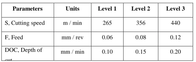
Table 3.2 Machining parameters and levels

Parameters Units Level 1 Level 2 Level 3

S, Cutting speed m / min 265 356 440

F, Feed mm / rev 0.06 0.08 0.12

DOC, Depth of

cut

mm / min 0.10 0.15 0.20

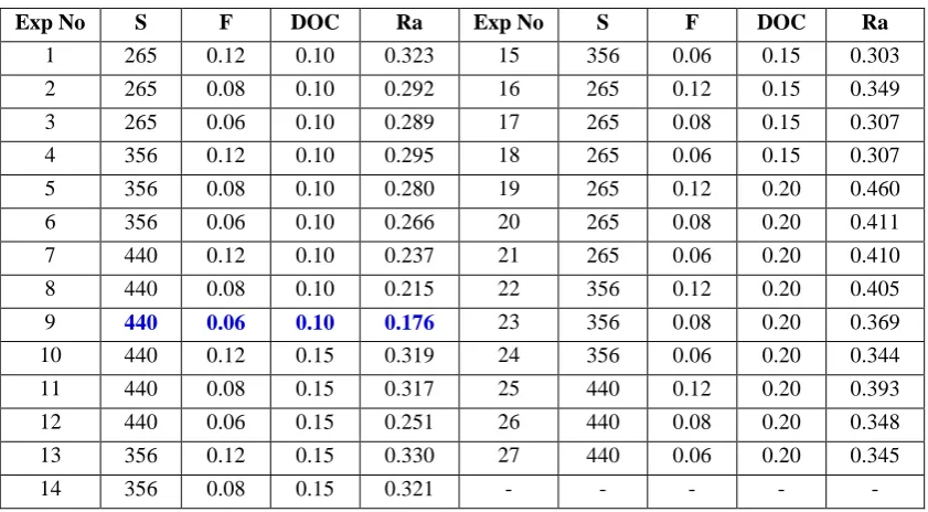
Taguchi L27 array was taken as the experimental plan. Atomic Force Microscope is utilized to measure the

261 | P a g e

Exp No S F DOC Ra Exp No S F DOC Ra

1 265 0.12 0.10 0.323 15 356 0.06 0.15 0.303

2 265 0.08 0.10 0.292 16 265 0.12 0.15 0.349

3 265 0.06 0.10 0.289 17 265 0.08 0.15 0.307

4 356 0.12 0.10 0.295 18 265 0.06 0.15 0.307

5 356 0.08 0.10 0.280 19 265 0.12 0.20 0.460

6 356 0.06 0.10 0.266 20 265 0.08 0.20 0.411

7 440 0.12 0.10 0.237 21 265 0.06 0.20 0.410

8 440 0.08 0.10 0.215 22 356 0.12 0.20 0.405

9 440 0.06 0.10 0.176 23 356 0.08 0.20 0.369

10 440 0.12 0.15 0.319 24 356 0.06 0.20 0.344

11 440 0.08 0.15 0.317 25 440 0.12 0.20 0.393

12 440 0.06 0.15 0.251 26 440 0.08 0.20 0.348

13 356 0.12 0.15 0.330 27 440 0.06 0.20 0.345

14 356 0.08 0.15 0.321 - - - - -

The relationship of the inputs vs. output variables are analysed with the Minitab17 software. First, second and

third order regression models are framed and compared for the statistical significance and the statistical values

of the equations are tabulated in Table 3.3.

Table 3.3 Regression model comparison for Surface roughness

Regression S R-sq R-sq

(adj)

R-sq (pred) Durbin - Watson

First order 0.02051 90.77% 89.56% 87.35% 1.46435

Second order 0.02105 92.81% 89.01% 81.38% 1.63960

Third order 0.010991 98.85% 97.00% 90.57% 2.58458

Third order regression R - sq values are the best than the first and second order regressions. While interpreting

the Durbin Watson values, of the third order regression is above 2 which indicate that the negative

autocorrelation. Durbin Watson value in the second order equations are lies between 1to 2 which indicates that

there is positive auto correlation between the predictors. Also the second order equation indicates that the

predictors (input variables) explain 92.81% of the variance in the output variables. The adjusted R - sq values

are close to the R - sq values which accounts for the number of predictors in the regression model. As both the

values together reveal that the model fits the data significantly. Finally the second order equation is preferred for

the examination and optimizing the parameters. Some set of values are generated with this regression equation.

262 | P a g e

The framed second order regression equations through the Minitab17 for the surface roughness in terms of

speed, feed and depth of cut combination are

Surface Roughness, “Ra = (0.331) – (0.000148*Speed) + (0.79*Feed) – (1.16*Depth of cut) –

(0.000001*Speed^2) – (4.0*Feed^2) + (5.56*Depth of cut^2) + (0.00100*Speed*Feed) + (2.40*Feed*Depth of

cut) + (0.00147*Speed*Depth of cut)”

(3.1)

By analyzing the coefficients of each input parameters the feed is contributing more influence on the surface

roughness comparing to the other two input variables.

IV. OPTIMIZATION METHODOLOGIES ADOPTED

The primary objective of this attempt is to investigate the intensity of the impact of the input parameters on the

surface roughness of the product and to forecast the optimal combination of the variables to attain the required

level of output. For that the optimisation technique selected is Particle Swarm optimisation which is one among

the popular algorithms being applied by many researchers. Initially the PSO algorithm is trained with the

experimented data in MATLAB programming by random selection of the input for data training with the

Gradient Descent with Momentum and Adaptive Learning. The mean squared error (MSE) is the indicator of the

simulation performance. The initial iteration was taken as 5000 turns and the outcome of the computation is

converged with 0.002767 mean error value. While increasing the number of iterations step by step and

evaluated, it is noticed that the employed PSO algorithm attains a steady rate of mean error as 0.000638 which shows 76.9 % improvement at 50000 turn’s iterations. Instead of taking the values at random, the simulation

programme was scheduled to take the regression equation relationship as input selection with the equated steps

263 | P a g e

surface roughness through experimented data are replaced with the values computed through regression

equation. On performing the simulation with these changes the results are found to be further tuned to the mean

error reduction (final mean error value is 0.00031). The pictorial representation of the newly proposed method is

shown in Fig. 4.1. The mean error comparison between each pahase of the method is focuesd through the Table

4.1.

Figure 4.1 Block diagram of Hybridization of Regression in PSO Algorithm

Table 4.1 Mean error comparison

Description PSO with Experimental data

PSO with Regression

Formula

PSO with Regression

values as input

Iterations 5000 50000 50000 50000

Mean error value 0.0027671 0.0006388 0.000361 0.00031

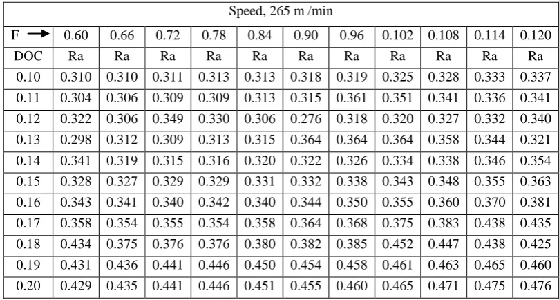
The step values given as input for simulation are as Speed = (265:17.5:440); Feed = (0.06:0.006:0.12); and

Depth of cut = (0.10:0.01:0.20). The simulated results through the method adopted are marked in the Table 4.2

and Table 4.3 for combination of speed, feed and depth of cut marked respectively.

Table 4.2 Iterated values of Ra for S 265 m / min, F 0.60 – 0.120 mm / rev and DOC 0.10 – 0.20 mm

Speed, 265 m /min

F 0.60 0.66 0.72 0.78 0.84 0.90 0.96 0.102 0.108 0.114 0.120

DOC Ra Ra Ra Ra Ra Ra Ra Ra Ra Ra Ra

0.10 0.310 0.310 0.311 0.313 0.313 0.318 0.319 0.325 0.328 0.333 0.337 0.11 0.304 0.306 0.309 0.309 0.313 0.315 0.361 0.351 0.341 0.336 0.341 0.12 0.322 0.306 0.349 0.330 0.306 0.276 0.318 0.320 0.327 0.332 0.340 0.13 0.298 0.312 0.309 0.313 0.315 0.364 0.364 0.364 0.358 0.344 0.321 0.14 0.341 0.319 0.315 0.316 0.320 0.322 0.326 0.334 0.338 0.346 0.354 0.15 0.328 0.327 0.329 0.329 0.331 0.332 0.338 0.343 0.348 0.355 0.363 0.16 0.343 0.341 0.340 0.342 0.340 0.344 0.350 0.355 0.360 0.370 0.381 0.17 0.358 0.354 0.355 0.354 0.358 0.364 0.368 0.375 0.383 0.438 0.435 0.18 0.434 0.375 0.376 0.376 0.380 0.382 0.385 0.452 0.447 0.438 0.425 0.19 0.431 0.436 0.441 0.446 0.450 0.454 0.458 0.461 0.463 0.465 0.460 0.20 0.429 0.435 0.441 0.446 0.451 0.455 0.460 0.465 0.471 0.475 0.476

Experimental data

Regression Modeling

Regression values

Particle Swarm

Optimization Simulated

264 | P a g e

Speed, 282.5 m /min

F 0.60 0.66 0.72 0.78 0.84 0.90 0.96 0.102 0.108 0.114 0.120

DOC Ra Ra Ra Ra Ra Ra Ra Ra Ra Ra Ra

0.10 0.311 0.313 0.318 0.316 0.320 0.323 0.325 0.332 0.332 0.338 0.341

0.11 0.309 0.314 0.314 0.317 0.367 0.356 0.346 0.336 0.330 0.338 0.361

0.12 0.311 0.351 0.333 0.312 0.285 0.319 0.325 0.328 0.332 0.334 0.341

0.13 0.353 0.315 0.315 0.361 0.353 0.348 0.347 0.346 0.340 0.320 0.348

0.14 0.338 0.324 0.323 0.326 0.324 0.331 0.331 0.337 0.342 0.390 0.318

0.15 0.333 0.329 0.331 0.334 0.333 0.339 0.343 0.344 0.350 0.356 0.364

0.16 0.341 0.344 0.345 0.341 0.345 0.349 0.351 0.356 0.363 0.371 0.378

0.17 0.358 0.358 0.357 0.356 0.358 0.364 0.369 0.374 0.429 0.427 0.457

0.18 0.428 0.432 0.372 0.373 0.375 0.382 0.443 0.437 0.422 0.401 0.411

0.19 0.427 0.432 0.437 0.441 0.445 0.448 0.450 0.451 0.452 0.448 0.433

0.20 0.427 0.432 0.437 0.441 0.445 0.449 0.453 0.458 0.460 0.459 0.454

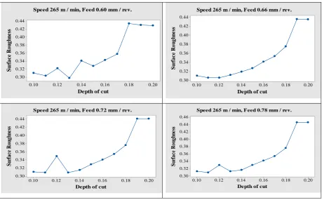
The graphical representation of the surface roughness with respect to the speed 265 m / min for all combination

of depth of cut and feed of 0.60 mm / rev to 0.78 mm/ rev are shown in the Fig. 4.2.

0.20 0.18 0.16 0.14 0.12 0.10 0.44 0.42 0.40 0.38 0.36 0.34 0.32 0.30

Depth of cut

S u rf a ce R o u g h n es s

Speed 265 m / min, Feed 0.60 mm / rev.

0.20 0.18 0.16 0.14 0.12 0.10 0.44 0.42 0.40 0.38 0.36 0.34 0.32 0.30

Depth of cut

S u rf a ce R o u g h n es s

Speed 265 m / min, Feed 0.66 mm / rev.

0.20 0.18 0.16 0.14 0.12 0.10 0.44 0.42 0.40 0.38 0.36 0.34 0.32 0.30

Depth of cut

S ur fa ce R ou gh ne ss

Speed 265 m / min, Feed 0.72 mm / rev.

0.20 0.18 0.16 0.14 0.12 0.10 0.46 0.44 0.42 0.40 0.38 0.36 0.34 0.32 0.30

Depth of cut

S ur fa ce R ou gh ne ss

Speed 265 m / min, Feed 0.78 mm / rev.

265 | P a g e

V

.

RESULTS AND CONCLUSIONS

Second order regression relationship is found to be fit with statistical significance. Feed is most contributing

input parameter which influences the surface roughness values highly comparing to the other two input

variables. PSO algorithm hybridization with regression relationship and regression computed values as input

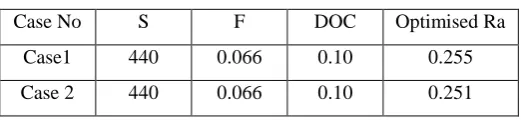
converges with minimum mean error. The optimised result for both the cases in individual simulation is

tabulated in the following Table 5.1.

Table 5.1 Optimised results

Case No S F DOC Optimised Ra

Case1 440 0.066 0.10 0.255

Case 2 440 0.066 0.10 0.251

Case 1 represents the regression relationship hybridization while case 2 represents the regression compute value

taken as input in the hybridization. The proposed hybridization method may be considered for future references

while compiling the optimisation of parameters in other process also. Manufacturers may use this as a

referenceset for their processing in order to select the optimal parameter combination according to the required

surface finish value to avoid the rework and part rejection. The analysis can be extended to find out the tool

wear, material removal rate, machining time, power consumption etc.

VI. RECOMMENDATIONS

The computed values of the regression relationship equations need to be examined and ensured for statistical

significance in all aspects while assigning as the input values for compiling. By selecting the steps value much

closer leads to get smoother curve fittings for references. the present graphical values may be taken as a ready

reckoner by the manufacturers for processing the parts. Attempts may be exercised with other familiar accepted

optimisation algorithms.

REFERENCES

[1] P V S. Suresh, K. Venkatehwara Rao and S G. Desmukh, A genetic algorithmic approach for optimization of

the surface roughness prediction model, International Journal of Machine Tools Manufacturing, 42, 2002,

675-680.

[2] A.Mital, M. Mehta, Surface roughness prediction models for fine turning, Int. J. Prod. Res, 26 (12), 1988,

1861-1876.

[3] M.A. El-Baradie, Surface roughness model for turning grey cast iron (154 BHN), Proceedings of the Institution of Mechanical Engineering, Part B, J. Eng. Manufac, 207 (B1), 1993, 43-54.

[4] El-Sonbaty and A.A. Megahed, On the prediction of surface roughness in turning using artificial neural

networks, Proceedings of the 7th Cairo University International ADP Conference, Cairo, Egypt, 2000, 455.

[5] M. Hasegawa, A. Seireg and R A. Lindberg, Surface roughness model for turning, Tribology Int, 9, 1976,

266 | P a g e

[6] Y. Sahin and A R. Motorcu, Surface roughness model for machining mild steel with coated carbide tool,

Mater Design, 26, 2005, 321-326.

[7] Y. Sahin and A R. Motorcu, Surface roughness model in machining hardened steel with cubic boron nitride

cutting tool, Int J Refract Met Hard Mater, 26, 2008, 84-90.

[8] G. Petropoulos, F. Mata and J. Paulo Davim, Statistical study of surface roughness in turning of peek

composites, Materials and Design, 29, 2008, 218-223.

[9] W. Grzesik and T. Wanat T, Surface finish generated in hard turning of quenched alloy steel parts using conventional and wiper ceramic inserts, Int J Mach Tools Manuf, 46, 2006, 1988-1995.

[10]W S. Lin, B Y. Lee and C L. Wu, Modeling the surface roughness and cutting force for turning, J Mater

Process Technol, 108, 2001, 286-293.

[11]A V. Gopal and P V. Rao, Selection of optimum conditions for maximum material removal rate with surface

finish and damage as constraints in SiC grinding, Int J Mach Tools Manuf, 43, 2003, 1327-1336.

[12]Nikolaos, Galanis, E. Dimitrios and Manolakos, Surface roughness prediction in turning of femoral head, Int

J Adv Manuf Technol, 51, 2010, 79-86.

[13]H. Singh and P. Kumar, Optimizing multi-machining characteristics through Taguchi’s approach and utility concept, Int. Jour. of MTM, 17, 2006, 36-45.

[14]J S. Agapiou, Design characteristics of new types of drill and evaluation of their performance drilling cast

iron. I. Drill with four major cutting edges, Int J Mach Tools Manuf, 33, 1993, 321-341.

[15]T. Oezel and Y. Karpat, Predictive modeling of surface roughness and tool wear in hard turning using

regression and neural networks, Int J Mach Tools Manuf, 45, 2005, 467-479.

[16]Emad Ellbeltagi, Tarek Hegazy and Donald Grierson, Comparison among five evolutionary – based

optimization algorithms, International Journal of Advanced Engineering Informatics, 19, 2005, 43-53.

[17]R. Saravanan, R. Sivasankar, P. Asokan. K. Vijayakumar and G. Prabhaharan, Optimization of cutting

conditions during continuous finished profile machining using non-traditional techniques, International

Journal of Advanced Manufacturing Technology, 26 (9), 2005, 1123-1128.

[18]B. Denkena, D. Boehnke, C. Spille and R Dragon, In-process information storage on surfaces by turning

operations, CIRP Annals - Manufacturing Technology, 57, 2008, 85-88.

[19]V. Achala, Dassanayake and C Steve Suh, On nonlinear cutting response and tool chatter in turning