Article
1
An Efficient Grid-based K-prototypes Algorithm for
2
Sustainable Decision Making using Spatial Objects
3
Hong-Jun Jang 1, Byoungwook Kim 2, Jongwan Kim 3 and Soon-Young Jung 4,*
4
1 Department of Computer Science and Engineering, Korea University, Seoul, 02841, Korea;
5
6
2 Department of Computer Engineering, Dongguk University, Gyeongju, 38066, Korea;
7
8
3 Smith Liberal Arts College, Sahmyook University, Seoul, 01795, Korea; [email protected]
9
4 Department of Computer Science and Engineering, Korea University, Seoul, 02841, Korea; [email protected]
10
* Correspondence: [email protected]; Tel.: +82-2-3290-2394
11
12
Abstract: Data mining plays a critical role in the sustainable decision making. The k-prototypes
13
algorithm is one of the best-known algorithm for clustering both numeric and categorical data.
14
Despite this, however, clustering a large number of spatial object with mixed numeric and
15
categorical attributes is still inefficient due to its high time complexity. In this paper, we propose an
16
efficient grid-based k-prototypes algorithms, GK-prototypes, which achieves high performance for
17
clustering spatial objects. The first proposed algorithm utilizes both maximum and minimum
18
distance between cluster centers and a cell, which can remove unnecessary distance calculation. The
19
second proposed algorithm as extensions of the first proposed algorithm utilizes spatial dependence
20
that spatial data tend to be more similar as objects are closer. Each cell has a bitmap index which
21
stores categorical values of all objects in the same cell for each attribute. This bitmap index can
22
improve the performance in case that a categorical data is skewed. Our evaluation experiments
23
showed that proposed algorithms can achieve better performance than the existing pruning
24
technique in the k-prototypes algorithm.
25
Keywords: clustering; spatial data; grid-based k-prototypes; data mining; sustainability
26
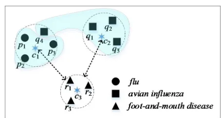
27
1. Introduction
28
Sustainability is a concept for balancing environmental, economic and social dimensions with
29
decision-making [23]. Data mining in sustainability is a very important issue since it sustainable
30
decision making contributes to the transition to a sustainable society [24]. Especially, there is a
31
growing interest in spatial data mining in making sustainable decisions in geographical
32
environments and national land policies [25].
33
Recently, spatial data mining has become more and more important as spatial data collection is
34
increasing due to technological developments such as geographic information system (GIS) and
35
global positioning system (GPS) [26][27]. The main techniques of spatial data mining are spatial
36
clustering [1], spatial classification [2], spatial association rule [3], and spatial characterization [4].
37
Spatial clustering is a technique used to classify data with high similar geographic and locational
38
characteristics into the same group. It is an important component to discover hidden knowledge in a
39
huge of spatial data [5]. Spatial clustering is used in the HotSpot detection which detects areas where
40
specific events occur [6]. Hotspot detection is used in various fields such as crime analysis [7,8,9], fire
41
analysis [10] and disease analysis [11,12,13,14].
42
Most spatial clustering studies have focused on efficiently finding groups for numeric data such
43
as location information of spatial objects. However, many real-world spatial objects have categorical
44
data, not just numeric data. Hence, if the categorical data affect spatial clustering results, the error
45
value can be increased when the final cluster results are evaluated.
46
47
48
Figure 1. An example of clustering using location information
49
We present an example of disease analysis clustered using only location information. Figure 1
50
shows 10 cases of disease location divided into three clusters. Diseases are divided into three
51
categories (i.e. p, q and r), and the measures to be taken in the area vary according to each disease. In
52
Figure 1, the representative attribute of cluster c1 is set to p, so we only deal with p. Therefore, when
53
q occurs in the same area, it is difficult to cope with. In this example, three clusters are constructed
54
using only numeric data (location information of disease occurrence). If the data from this example
55
was used to inform a policy decision, it could result in a decision maker failing to implement the
56
correct policy.
57
Data generated in the real world is often mixed with numeric data as well as categorical data. In
58
order to apply the clustering technique to the real world, algorithms that can consider categorical
59
data are required. A representative clustering algorithm that can use mixed data is the k-prototypes
60
algorithm [15]. The basic k-prototypes algorithm has a large time complexity due to the processing
61
of all data. Therefore, it is important to reduce execution time in order to process the k-prototypes
62
algorithm on large data. However, only a few studies have been conducted to reduce the time
63
complexity of the k-prototypes algorithm. Kim [16] proposed a pruning technique to reduce distance
64
computation between an object and cluster centers using the concept of partial distance computation.
65
However, this method does not have high pruning efficiency by comparing objects one by one with
66
cluster center.
67
To improve performance, we propose an effective grid-based k-prototypes algorithm,
GK-68
prototypes, for clustering spatial objects. The proposed method makes use of the grid-based indexing
69
technique which improve pruning efficiency to compare distance between cluster centers and a cell
70
instead of cluster centers and an object.
71
Spatial data can have geographic data as categorical attributes that indicate the characteristics of
72
the object as well as the location of the object. Geographic data tend to have spatial dependence.
73
Spatial dependence is the property of objects that are close to each other having increased similarities
74
[17]. For example, soil types or network type are more likely to be similar at points one meter apart
75
than at points one kilometer apart. Due to the nature of spatial dependence, the categorical data of
76
spatial data is often skewed according to the position of the object. For improving performance of a
77
grid-based k-prototypes algorithm, we take advantage of the spatial dependence to the bitmap
78
indexing technique.
79
The contributions of this paper are summarized as follows.
80
We proposed an effective grid-based k-prototypes, GK-prototypes, which improve the
81
performance of a basic k-prototypes algorithm.
82
We developed a pruning technique which utilizes the minimum and maximum distance on
83
numeric attributes and the maximum distance on categorical attributes between a cell and a
84
cluster center.
85
We developed a pruning technique based on a bitmap index to improve the efficiency of the
86
pruning in case that a categorical data is skewed.
87
We conducted several experiments on synthetic datasets. Our algorithms can achieve better
88
The organization of the rest of this paper is as follows. In Section 2, the basic k-prototypes
90
algorithm and the previous research on pruning in the k-prototypes algorithm are described. In
91
Section 3, we first briefly describe some basic notations and definitions. After that, the proposed
GK-92
prototypes algorithm is explained in Section 4. In Section 5, experimental results on synthetic data
93
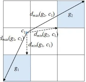
demonstrate the performance. Section 6 concludes the paper.
94
2. Related works
95
2.1. The k-prototypes algorithm
96
The k-prototypes algorithm is first proposed clustering algorithm to deal with mixed data types
97
(numeric data and categorical data), which integrates k-means and k-modes algorithms [15]. Let a set
98
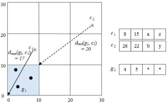
of n objects be O={o1, o2, …, on} where oi=(oi1, oi2, …, oim) is consisted of m attributes. The purpose of
99
clustering is to partition n objects into k disjoint clusters C={C1, C2, …, Cn} according to the degree of
100
similarity of objects. The distance is used as a measure to group objects with high similarity into the
101
same cluster. The distance d(oi, Cj) between oi and Cj is calculated as follows:
102
d(oi, Cj) = dr(oi, Cj) + dc(oi, Cj) (1)
where d
r(o
i, C
j) is the distance between numeric attributes and d
c(o
i, C
j) is the distance
103
between categorical attributes.
104
, = − (2)
, = , (3)
, = 0, ℎ =
1, ℎ ≠ (4)
In Equation (2), dr(oi, Cj) is the squared Euclidean distance between an object and a cluster center
105
on the numeric attributes. dc(oi, Cj) is the dissimilar distance on the categorical attributes, where oik
106
and cjk, 1≤k≤p, are values of numeric attributes, oik and cjk, p+1≤k≤m are values of categorical attributes.
107
That is, p is the number of numeric attributes and m-p is the number of categorical attributes.
108
2.2. Existing pruning technique in the k-prototypes algorithm
109
The k-prototypes algorithm spends most of execution time computing the distance between an
110
object and cluster centers. In order to improve the performance of the k-prototypes algorithm, Kim
111
[16] proposed the concept of partial distance computation (PDC) which compares only partial
112
attributes, not all attributes in measuring distance. The maximum distance that can be measured in
113
one categorical attribute is 1. Thus the distance that can be measured from the categorical attributes
114
is bound to the number of categorical attributes, m-p. Given an object o and the two cluster centers (c1
115
and c2), if the difference between dr(o, c1) and dr(o, c2) is more than m-p, we can know which clusters
116
are closer to the object without the distance using the categorical attributes. However, PDC is still not
117
efficient due to the fact that all objects are involved in the distance calculation and the characteristic
118
(i.e. spatial dependence) of spatial data is not utilized in the clustering process.
119
2.3. Grid-based clustering algorithm
120
The grid-based techniques have the fastest processing time that depends on the number of the
121
grid cells instead of the number of objects in the data set [18]. The basic grid-based algorithm is as
122
follows. At first, a set of grid-cells is defined. In general, these grid-based clustering algorithm use a
123
single uniform or multi-resolution grid cell to partition the entire datasets into cells. Each object is
124
degree of density is below a certain threshold, are eliminated. In addition to the density of cells,
126
statistical information of objects in the cell is computed. After that, the clustering process is performed
127
on the grid cells using each cell’s statistical information, instead of the objects itself.
128
The representative grid-based clustering algorithms are STING [19] and CLIQUE [20]. STING is
129
a grid-based multi resolution clustering algorithm in which the spatial area is divided into
130
rectangular cells with a hierarchical structure. Each cell at a high level is divided into several smaller
131
cells in the next lower level. For each cell in pre-selected layer, the relevancy of the cell is checked by
132
computing the confidence interval. If the cell is relevant, we include the cell in a cluster. If the cell is
133
irrelevant, it is removed from further consideration. We look for relevant cells at the next lower layer.
134
This algorithm combines relevant cells into relevant regions and return the so obtained clusters.
135
CLIQUE is a grid-based and density-based clustering algorithm to identify subspaces of a high
136
dimensional data that allow better clustering quality than original data. CLIQUE partitions the
n-137
dimensional data into non overlapping rectangular units. The units are obtained by partitioning
138
every dimension into certain intervals of equal length and selectivity of a unit is defined as the total
139
data points contained in it. A cluster in CLIQUE is a maximal set of connected dense units within a
140
subspace. In a grid-based clustering study, the grid is used in order that clustering is performed on
141
the grid cells, instead of objects itself. Chen et al. [21] proposes algorithm called GK-means, which
142
integrates grid structure and spatial index with k-means algorithm. It focuses on choice the better
143
initial centers to improve the clustering quality and to reduce the computational complexity of
k-144
means.
145
Most existing grid-based clustering algorithms regard objects in same cell of grid as a data point
146
to process large scale data. Thus, the final clustering results of these algorithms are not the same as a
147
basic k-prototype cluster result, but all the cluster boundaries are either horizontal or vertical. In
GK-148
means, the grid is used to select initial centers and remove noise data, but not used to reduce
149
unnecessary distance calculation. To the best of our knowledge, such a grid-based pruning technique
150
to improve the performance of the k-prototypes algorithm has not been previously demonstrated.
151
3. Preliminary
152
In this section, we present some basic notations and definitions before describing our algorithms.
153
We summarize the notation used throughout this paper in Table 1.
154
Table 1. A summary of notations
155
Notation Description
O a set of data oi i-th data in O
n the number of objects
m the number of attributes of an object ci the i cluster center point
vi the value of grid partition interval gk a cell of grid
d(oi, cj) a distance between an object and an cluster center
dr(oi, cj) a distance between an object and an cluster center for only numeric attributes dc(oi, cj) a distance between an object and an cluster center for only categorical attributes dmin(gi, cj) the minimum distance between a cell and a cluster center for only numeric
attributes
dmax(gi, cj) the maximum distance between a cell and a cluster center for only numeric attributes
156
Consider a set of n objects, O={o1, o2, …, on}. oi=(oi1, oi2, …, oim) is an object represented by m
157
attribute values. The m attributes consist of mr (the number of numeric attributes) and mc (the number
158
calculated by Equation (1) in Section 2. We adopt the data indexing technique based on grid for
160
pruning. First we define the cells that make up the grid.
161
162
Definition 1. A cell g in mr-dimension grid is defined by a start point vector S and an end point vector
163
T: g = (S, T), where S = [s1, s2, …, smr] and T = [t1, t2, …, tmr] and si ≤ ti for 1 ≤ i ≤ mr and si + vi = ti. The vi
164
is interval distance between start and end position of a cell g on i-dimension.
165
166
Definition 2. The minimum distance between a cell gi and a cluster center cj for numeric attributes,
167
denoted dmin(gi, cj), is;
168
dmin(gi, cj) = ∑ | − | ,
169
where =
< >
ℎ .
170
We use the classic Euclidian distance to measure the distance. If a cluster center is inside the cell,
171
the distance between them is zero. If a cluster center is outside the cell, we use the Euclidean distance
172
between the cluster center and the nearest edge of the cell.
173
174
Definition 3. The maximum distance between a cell gi and a cluster center cj for numeric attributes,
175
denoted dmax(gi, cj), is;
176
dmax(gi, cj)= ∑ | − | ,
177
where = , ≤
, ℎ .
178
To distinguish between the two distances dmin and dmax, an example is illustrated in Figure 2,
179
showing a cluster center (c1), two cells (g1 and g2) and the corresponding distances.
180
181
182
Figure 2. An example of distances dmin and dmax.
183
In a grid-based approach, dmin(g,c) and dmax(g,c) for a cell g and cluster centers c, are measured
184
firstly before measuring the distance between an object and cluster centers. We can use dmin and dmax
185
to improve performance of k-prototypes algorithm. Figure 3 shows an example of pruning using dmin
186
188
Figure 3. An example of pruning method using minimum distance and maximum distance
189
In Figure 3, the maximum distance between g1 and c1, dmax(g1, c1) = 17( (8 − 0) + (15 − 0)). The
190
minimum distance between g1 and c2, dmin(g1, c2) = 20 ( (26 − 10) + (22 − 10)). The dmax(g1, c1) is three less than
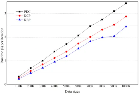
191
dmin(g1, c2). Therefore, all objects in g1 are closer to c1 than c2, if we are considering only numeric
192
attributes. To find the closest cluster center from an object, we have to measure the distance by
193
categorical attributes. If the difference between dmin and dmax is more than mc (maximum distance by
194
categorical attributes), however, the cluster closest to the object can be determined without the
195
distance by categorical attributes. In Figure 3, the categorical data of c1 is (a, z), and the categorical
196
data of c2 is (b, y). Assume that there are no objects in g1 with ‘a’ in the first categorical attribute and
197
‘z’ in second categorical attribute. Since dc(o, c1) of all objects in g1 is 2, maximum distance of all objects
198
in g1 is dmax(g1, c1) + 2. The maximum distance between c1 and objects in g1 is not less than the minimum
199
distance between c2 and objects in g1. We can know that all objects in g1 are closer to c1 than c2.
200
201
Lemma 1. For any cluster centers ci, cj and any cell gx, if dmin(gx, cj) - dmax(gx, ci) > mc then, ∀o∈gx, d(o, ci)
202
< d(o, cj).
203
Proof. By assumption, dmin(gx, cj) > mc + dmax(gx, ci). By Definition 2 and 3, dmin(gx, ci)≤d(ci, o)≤dmax(gx, ci)+mc,
204
and dmin(gx, cj)≤d(cj, o)≤dmax(gx, cj)+mc. d(ci, o)≤dmax(gx, ci)+m<dmin(gx, cj)≤d(cj, o). ∴∀o∈gx, d(ci, o) < d(cj, o) □.
205
206
Lemma 1 is the basis for our proposed pruning techniques. In the process of clustering, we first
207
exploit Lemma 1 to remove cluster centers to be compared to objects.
208
4. GK-prototypes algorithm
209
In this section, we present two pruning techniques that are based on grid for improving the
210
performance of the k-prototypes algorithm. The first pruning technique is KCP (K-prototypes
211
algorithm with Cell Pruning) which utilizes dmin, dmax and the maximum distance on categorical
212
attributes. The second pruning technique is KBP (K-prototypes algorithm with Bitmap Pruning)
213
which utilizes bitmap indexes to reduce unnecessary distance calculation on categorical attributes.
214
4.1. Cell pruning technique
215
The computational cost of the k-prototypes algorithm is most often encountered in the step of
216
measuring distance between objects and cluster centers. To improve the performance, each object is
217
indexed into a grid by numeric data in data preparation step. We set up grid cells storing two types
218
of information. a) The first is a start point vector S and an end point vector T, which is the range of
219
the numeric value of the objects to be included in the cell (see Definition 1). Based on this cell
220
information, the minimum and maximum distances between each cluster centers and a cell are
221
measured. b) The second is bitmap indexes which is explained in Subsection 4.2.
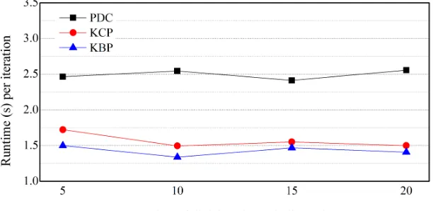
222
Algorithm 1 The k-prototypes algorithm with cell pruning (KCP)
224
Input: k: the number of cluster, G: the grid in which all objects are stored per cell
225
Output: k cluster centers
226
1: C[ ]← Ø // k cluster centers
227
2: Randomly choosing k object, and assigning it to C.
228
3: while IsConverged() do
229
4: for each cell g in G
230
5: dmin[ ], dmax[ ] ← Calc(g, C)
231
6: dminmax ← min(dmax[ ])
232
7: candidate ← Ø
233
8: for j ←1 to k do
234
9: if (dminmax + mc > dmin[j] ) // Lemma 1
235
10: candidate ← candidate ∪ j
236
11: end for
237
12: min_distance ← ∞
238
13: min_cluster ← null
239
14: for each object o in g
240
15: for each center c in candidate
241
16: if min_distance > d(o, c)
242
17: min_cluster ← index of c
243
18: end for
244
19: Assign(o, min_cluster)
245
20: UpdateCenter(C[c])
246
21: end for
247
22: end while
248
23: return C[k]
249
250
The details of the cell pruning are as follows. First, we initialize an array C[j] to store the position
251
of k cluster centers, 1≤j≤k. Various initial cluster centers selection methods have been studied to
252
improve the accuracy of clustering results in the k-prototypes algorithm [22]. Since we aim at
253
increasing the clustering speed improvement, however, we adopt a simple method to select k objects
254
randomly from input data and use them as initial cluster centers.
255
In general, the result of clustering algorithm is evaluated after a single clustering process has
256
been performed. Based on these evaluation result, it is determined whether the same clustering
257
process have to be repeated or terminated. The iteration is terminated if the sum of the difference
258
between the current cluster center and the previous cluster center is less than a predetermined value
259
(ε) as an input parameter by users. In Algorithm 1, we determine the termination condition through
260
the IsConverged() function of the while statement.
261
In iteration step of clustering (line 4), the distances between objects and k cluster centers are
262
measured by cells. The Calc(g, C) function returns the minimum and maximum distances between a
263
cell g and k cluster centers (C) for each cluster center (line 5). The smallest distance among the
264
maximum distance is stored in the dminmax (line 6). The candidate stores the index number of the
265
cluster center that need to be measured from the cell. Through Lemma 1, if dminmax+mc is greater
266
than dmin[j], the j cluster center is included in the distance calculation, otherwise it is excluded (lines
267
8-11). After Lemma 1 is applied, only the cluster centers to be measured the distance from objects in
268
the cell are finally left in the candidate. All objects in the cell are measured from the cluster centers in
269
the candidate, d(o, c), (line 16). An object is assigned to the cluster where d(o, c) is computed as the
270
smallest value using Assign(o, min_cluster) function. The center of cluster to which a new object is
271
added is updated by remeasuring its cluster center using UpdateCenter(C[c]) function. This clustering
272
4.2. Bitmap pruning technique
274
Spatial data tend to have similar categorical values in neighboring objects, categorical data is
275
often skewed. If we can utilize the characteristics of spatial data, the performance of the k-prototypes
276
algorithm can be further improved. In this subsection, we introduce the KBP that can improve the
277
efficiency of pruning when categorical data is skewed.
278
The KBP stores categorical data of all objects in a cell in a bitmap index. Figure 4 shows an
279
example of storing categorical data as a bitmap index. Figure 4(a) is an example of spatial data. The
280
x and y attributes indicate location information of objects as numeric data, and z and w attributes
281
indicate features of objects as categorical data. For five objects in the same cell, g={o1, o2, o3, o4, o5},
282
Figure 4(b) shows the bitmap index structure where a row presents a categorical attribute and a
283
column presents a categorical data of objects in same cell. A bitmap index consists of one vector of
284
bits per attribute value, where the size of each bitmap is equal to the number of categorical data in
285
the raw data. The bitmaps are encoded such that the i-th bit is set to 1 if the raw data has a value
286
corresponding to the i-th column in the bitmap index, otherwise it is set to 0. For example, the value
287
1 in z row and c column from bitmap index means that the value c exists in z attribute of raw data.
288
When raw data is converted to a bitmap index, object id information is removed. We can quickly
289
check for the existence of the specified value in raw data using the bitmap index.
290
291
292
Figure 4. Bitmap indexing structure
293
A maximum of categorical distance is determined by the number of categorical attributes (mc).
294
If the difference of two numeric distance between one object and two cluster centers, |dr(o, ci) - dr(o,
295
cj)|, is more than mc, we can know the cluster center closer to the object without categorical distance.
296
However, since the numeric distance is not known in advance, we cannot determine the cluster center
297
closer to the object by only categorical distance. Thus, the proposed KBP is utilized in reducing
298
categorical distance calculations in the KCP. Algorithm 2 describes the proposed KBP. We explain
299
only the extended parts from the KCP.
300
301
Algorithm 2 The k-prototypes algorithm with bitmap pruning (KBP)
302
Input: k: the number of cluster, G: the grid in which all objects are stored per cell
303
Output: k cluster centers
304
1: C[k]← Ø // k cluster center
305
2: Randomly choosing k object, and assigning it to C.
306
3: while IsConverged() do
307
4: for each cell g in G
308
5: dmin[], dmax[] ← Calc(g, C)
309
6: dminmax ← min(dmax[])
310
7: arrayContain[] ← IsContain(g, C)
311
8: candidate ← Ø
312
9: for j ←1 to k do
313
11: candidate ← candidate ∪ j
315
12: end for
316
13: min_distance ← ∞
317
14: min_cluster ← null
318
15: distance ← null
319
16: for each object o in g
320
17: for each center c in candidate
321
18: if (arrayContain [c] == 0)
322
19: distance = dr(o, c) + mc
323
20: else
324
21: distance = dr(o, c) + dc(o, c)
325
22: if min_distance > distance
326
23: min_cluster ← index of cluster center
327
24: end for
328
25: Assign(o, min_cluster)
329
26: UpdateCenter(C)
330
27: end for
331
28: end while
332
29: return C[k]
333
334
To improve the efficiency of pruning on categorical data, the KBP is implemented by adding
335
two step to the KCP. The first step is to find out whether the categorical attributes value of each cluster
336
centers exists in the bitmap index of the cell using the IsContain function (line 7). The IsContain
337
function compares the categorical data of each cluster center with the bitmap index and returns 1 if
338
there is more than one of the same data in the corresponding attribute. Otherwise, it returns 0. In
339
Figure 4 (b), assume that we have a cluster center, ci = (2, 5, D, A). The bitmap index does not have D
340
in the z attribute and A in the w attribute. In this case, we can know that there are no objects in the
341
cell that have D in the z attribute and A in the w attribute. Therefore, the maximum categorical
342
distance between all objects belonging to a cell and cluster center ci is 0. Assume that we have another
343
the cluster center, cj = (2, 5, A, B). The bitmap index has A in the z attribute and B in the w attribute.
344
In this case, we can know that there are some objects in the cell that have A in the z attribute or b in
345
the w attribute. If one or more objects with the same categorical value are found in the corresponding
346
attribute, the categorical distance calculation has to be performed for all objects in the cell in order to
347
know the correct categorical distance. Finally, arrayContain[i] stores the result of the comparison
348
between the i-th cluster center and the cell. In lines 8-12, the cluster centers that need to measure
349
distance with each cell g are stored in the candidate like as the KCP. The second extended part (lines
350
18-23) is used to determine whether to measure the categorical distance using arrayContain. If
351
arrayContain[i] has 0, the mc is directly used as the result of the categorical distance without measuring
352
the categorical distance (line 19).
353
5. Experiments
354
In this section, we evaluate the performance of the proposed GK-prototypes algorithms. For
355
performance evaluation, we compare partial distance computation pruning (PDC) [16] and our two
356
algorithms (KCP and KBP). We examined the performance of our algorithms as the number of objects,
357
the number of clusters, the number of categorical attributes and the number of division in each
358
dimension increased. In Table 2, the parameters used for the experiments are summarized. The
359
rightmost column of the table means the baseline values of the various parameters. For each set of
360
parameters, we perform 10 sets of experiments and the average values are reported. Even under the
361
Therefore, we measure the performance of each algorithm with the average execution time that it
363
takes for clustering to repeat once.
364
Table 2. Parameters for the experiments
365
Parameter Description Baseline Value
n no. of objects 1,000K
k no. of clusters 10
mr no. of numeric attributes 2
mc no. of categorical attributes 5
s no. of division in each dimensions 10
366
The experiments are carried out on a PC with Intel(R) Core(TM) i7 3.5 GHz, 32GB RAM. All the
367
algorithms are implemented in Java.
368
5.1. Data sets
369
We generate many synthetic datasets with numeric attributes and categorical attributes. For
370
numeric attributes in each dataset, two numeric attributes are generated in the 2D space [0, 100]×[0,
371
100] to indicate an object’s location. Each object is assigned into s×s cells in a grid by these numeric
372
data. The numeric data is generated according to uniform distributions in which each numeric data
373
is selected in [0, 100] randomly or Gaussian distributions with mean = 50 and standard deviation =
374
10. The categorical data is generated according to uniform distributions or skewed distributions. For
375
uniform distributions, we select an alphabet from A to Z randomly. For skewed distributions, we
376
generate categorical data in such a way that objects in same cell have similar alphabet based on its
377
numeric data.
378
5.2. Effects of the number of objects
379
To illustrate scalability, we vary the number of objects from 100K to 1,000K. Other parameters
380
are given their baseline values (Table 2). Figures 5, 6 and 7 show the effect of the number of objects.
381
Three graphs are shown in a linear scale. For each algorithm, the runtime per iteration is
382
approximately proportional to the number of objects.
383
In Figure 5, KBP and KCP outperforms PDC. However, there is little difference in the
384
performance between KBP and KCP. This is because if the categorical data is uniform distribution,
385
most of the categorical data exist in the bitmap index. In this case, KBP is the same performance as
386
KCP.
387
388
Figure 5. Effect of the number of objects (numeric data and categorical data are on uniform
389
391
In Figure 6, KBP outperforms KCP and PDC. For example, KBP runs up to 1.1 and 1.75 times
392
faster than KCP and PDC, respectively (n=1,000K). If categorical data is on a skewed distribution,
393
KBP is effective for improving performance. As the size of the data increases, the difference in
394
execution time increases. This is because as the data size increases, the amount of distance calculation
395
increases, while at the same time the number of objects included in the cluster being pruned increases.
396
In Figure 7, KCP outperforms PDC. Even if numeric data is on a Gaussian distribution, cell pruning
397
is effective for improving performance.
398
399
Figure 6. Effect of the number of objects (numeric data is on uniform distribution and categorical data
400
is on skewed distribution)
401
402
Figure 7. Effect of the number of objects (numeric data is on Gaussian distribution and categorical
403
data is on skewed distribution)
404
5.3. Effects of the number of clusters
405
To confirm the effects of the number of clusters, we vary the number of clusters, k, from 5 and
406
20. Other parameters are kept at their baseline values (Table 2). Figures 8, 9 and 10 show the effects
407
of the number of clusters. Three graphs are also shown in a linear scale. For each algorithm, the
408
runtime is approximately proportional to the number of cluster.
409
In Figure 8, KBP and KCP also outperform PDC. However, there is also little difference in the
410
performance between KBP and KCP. This is because if the categorical data is uniform distribution,
411
most of the categorical data exist in the bitmap index like Figure 5.
412
414
Figure 8. Effect of the number of clusters (numeric data and categorical data are on uniform
415
distribution)
416
In Figure 9, KBP outperforms KCP and PDC. For example, KBP runs up to 1.13 and 1.71 times
417
faster than KCP and PDC, respectively (k = 10). This result indicates that KBP is effective for
418
improving performance even if categorical data is on a skewed distribution. As the number of cluster
419
increases, the difference in execution time increases. This is also because as the data size increases,
420
the amount of distance calculation increases, while at the same time the number of objects included
421
in the cluster being pruned increases like Figure 6. In Figure 10, KCP also outperforms PDC. Even if
422
numeric data is on a Gaussian distribution, KCP is also effective for improving performance.
423
424
Figure 9. Effect of the number of clusters (numeric data and categorical data are on uniform
425
distribution)
426
427
Figure 10. Effect of the number of clusters (numeric data is on Gaussian distribution and categorical
428
data is on skewed distribution)
429
5.4. Effects of the number of categorical attributes
431
To confirm the effects of the number of categorical attributes, we vary the number of categorical
432
attributes from 5 to 20. Other parameters are given their baseline values. Figure 11 shows the effect
433
of the number of categorical attributes. The graph is also shown in a linear scale. For each algorithm,
434
the runtime per iteration is approximately proportional to the number of categorical attributes. KBP
435
outperforms KCP and PDC. For example, KBP runs up to 1.13 and 1.71 times faster than KCP and
436
PDC, respectively (mc=5). Even if the number of the categorical attributes increases, the difference
437
between the execution time of KCP and PDC is kept almost constant. The reason is that KCP is based
438
on numeric attributes and is not affected by the number of categorical attributes.
439
440
441
Figure 11. Effect of the number of categorical attributes on a skewed distribution
442
5.5. Effects of the size of cells
443
To confirm the effects of the size of cells, we vary the number of cells from 5 to 20. Other
444
parameters are given their baseline values (Table 2). Figure 12 shows the effect of the number of
445
divisions in each dimension. KBP and KCP outperform PDC. In Fig. 13, the horizontal axis is the
446
number of divisions of each dimension. As the number of divisions increases, the size of the cell
447
decreases. As the cell size gets smaller, the distance between the cell and cluster centers can be
448
measured more finely. There is no significant difference in execution time according to the size of cell
449
by each algorithm. This is because the distance calculation between the cell and the cluster centers is
450
increased in proportion to the number of cells, and the bitmap index stored by the cell is also
451
increased.
452
453
Figure 12. Effect of the number of cells on a skewed distribution
454
6. Conclusions
456
In this paper we have propose an efficient grid-based k-prototypes algorithm, GK-prototypes,
457
that improves performance for clustering spatial objects. We develop two pruning techniques, KCP
458
and KBP. KCP which uses both maximum and minimum distance between cluster centers and a cell
459
improves the performance than PDC. KBP is an extension of cell pruning for improving the efficiency
460
of pruning in case that a categorical data is skewed. Our experimental results demonstrate that KCP
461
and KBP outperforms PDC, and KBP outperforms KCP except for uniform distributions of categorical
462
data. These results lead us to conclude that our grid-based k-prototypes algorithm can achieve better
463
performance than the existing k-prototypes algorithm.
464
As data has grown exponentially and more complex recently, the traditional clustering
465
algorithms have a great challenge to deal with these data. In future works, we may consider
466
optimized pruning techniques of the k-prototypes algorithm in parallel processing environment.
467
Author Contributions: Conceptualization, Hong-Jun Jang and Byoungwook Kim; Methodology, Hong-Jun
468
Jang; Software, Byoungwook Kim; Writing-Original Draft Preparation, Hong-Jun Jang and Byoungwook Kim;
469
Writing-Review & Editing, Jongwan Kim; Supervision, Soon-Young Jung.
470
Acknowledgments: This research was supported by Basic Science Research Program through the National
471
Research Foundation of Korea(NRF) funded by the Ministry of Education(No. NRF-2017R1D1A1B03034067) and
472
by the National Research Foundation of Korea(NRF) grant funded by the Korea government(MSIT) (No.
NRF-473
2016R1A2B1014013)
474
Conflicts of Interest: The authors declare no conflict of interest.
475
References
476
1. Sander, J.; Ester, M.; Kriegel, H.P.; Xu, X. Density-Based Clustering in Spatial Databases: The Algorithm
477
GDBSCAN and Its Applications. Data Mining and Knowledge Discovery 1998, 2, 169–194.
478
2. Koperski, K.; Han, J.; Stefanovic, N. An Efficient Two-Step Method for Classification of Spatial Data. In
479
Proceedings of the International Symposium on Spatial Data Handling (SDH'98), Vancouver, Canada, 1998,
480
pp. 45–54.
481
3. Koperski, K.; Han. J. (1995). Discovery of Spatial Association Rules in Geographic Information Databases.
482
In Proceedings of the 4th International Symposium on Advances in Spatial Databases (SSD'95), 1995, pp.
483
47–66.
484
4. Ester, M.; Frommelt, A.; Kriegel, H.P.; Sander, J. Algorithms for Characterization and Trend Detection in
485
Spatial Databases. In Proceedings of the Fourth International Conference on Knowledge Discovery and
486
Data Mining (KDD'98), 1998, pp. 44–50.
487
5. Deren, L.; Shuliang, W.; Wenzhong, S.; Xinzhou, W. On Spatial Data Mining and Knowledge Discovery.
488
Geomatics and Information Science of Wuhan Univers 2001, 26, 491–499.
489
6. Boldt, M.; Borg, A. A statistical method for detecting significant temporal hotspots using LISA statistics. In
490
Proceedings of the Intelligence and Security Informatics Conference (EISIC), 2017 European, 2017.
491
7. Chainey, S.; Reid, S.; Stuart, N. When is a Hotspot a Hotspot? A Procedure for Creating Statistically Robust
492
Hotspot Maps of Crime. In Innovations in GIS 9: Socio-economic applications of geographic information
493
science, Kidner, D; Higgs, G; White, S, Eds.; Taylor & Francis: London, UK, 2002; pp. 21–36.
494
8. Murray, A.; McGuffog, I.; Western, J.; Mullins, P. Exploratory spatial data analysis techniques for
495
examining urban crime. The British Journal of Criminology 2001, 41, pp. 309–329.
496
9. Chainey, S.; Tompson, L.; Uhlig, S. The Utility of Hotspot Mapping for Predicting Spatial Patterns of Crime.
497
Security Journal 2008, 21, pp. 4–28.
498
10. Di Martino, F.; Sessa, S. The extended fuzzy C-means algorithm for hotspots in spatio-temporal GIS. Expert
499
Systems with Applications 2011, 38, pp. 11829–11836.
500
11. Di Martino, F.; Sessa, S.; Barillari, U.E.S.; Barillari, M.R. Spatio-temporal hotspots and application on a
501
disease analysis case via GIS. Soft Computing 2014, 18, pp. 2377–2384.
502
12. Mullner, R.M.; Chung, K.; Croke, K. G.; Mensah, E. K. Geographic information systems in public health
503
and medicine. Journal of Medical Systems 2004, 28, pp. 215–221.
504
13. Polat, K. Application of attribute weighting method based on clustering centers to discrimination of
505
14. Wei, C.K.; Su, S.; Yang, M.C. Application of data mining on the development of a disease distribution map
507
of screened community residents of taipei county in Taiwan. Journal of Medical Systems 2012, 36, pp. 2021–
508
2027.
509
15. Huang, Z. Clustering large data sets with mixed numeric and categorical values. In Proceedings of the First
510
Pacific Asia Knowledge Discovery and Data Mining Conference, 1997, pp. 21–34.
511
16. Kim, B. A Fast K-prototypes Algorithm Using Partial Distance Computation. Symmetry 2017, 9,
512
doi:10.3390/sym9040058
513
17. Goodchild, M. Geographical information science. International Journal of Geographic Information Systems
514
1992, 6, pp. 31–45.
515
18. Xiaoyun, C.; Yi, C.; Xiaoli, Q.; Min, Y.; Yanshan, H. PGMCLU: a novel parallel grid-based clustering
516
algorithm for multi-density datasets. In: 1st IEEE symposium on web society, 2009 (SWS’09), Lanzhou,
517
2009, pp 166–171.
518
19. Wang, W.; Yang, J.; Muntz, R. R. STING: A Statistical Information Grid Approach to Spatial Data Mining.
519
In the 23rd International Conference on Very Large Data Bases (VLDB’97), 1997, pp. 186–195.
520
20. Agrawal, R.; Gehrke, J.; Gunopulos, D.; Raghavan, P. Automatic Subspace Clustering of High Dimensional
521
Data for Data Mining Applications. In Proceedings of the ACM SIGMOD International Conference on
522
Management of Data, ACM Press, 1998, pp. 94–105.
523
21. Chen, X., Su, Y., Chen, Y., & Liu, G. GK-means: An Efficient K -means Clustering Algorithm Based On Grid.
524
In Computer Network and Multimedia Technology (CNMT 2009) International Symposium, 2009.
525
22. Ji, J.; Pang, W.; Zheng, Y.; Wang, Z.; Ma, Z.; Zhang, L. A Novel Cluster Center Initialization Metho
526
d for the k-Prototypes Algorithms using Centrality and Distance. Applied Mathematics & Information
527
Sciences 2015, 9, pp. 2933–2942.
528
23. Zavadskas, E.K.; Antucheviciene, J.; Vilutiene, T.; Adeli, H. Sustainable Decision Making in Civil Enginee
529
ring, Construction and Building Technology. Sustainability 2018, 10, 14.
530
24. Hersh, M.A. Sustainable Decision Making: The Role of Decision Support systems. IEEE Transactions on Sy
531
stems, Man, and Cybernetics-Part C: Applications and Reviews 1999, 29, 3, pp. 395-408.
532
25. Morik, K.; Bhaduri, K.; Kargupta. H. Introduction to data mining for sustainability. Data Mining and
533
Knowledge Discovery 2012, 24, 2, pp. 311-324.
534
26. Aissi, S.; Gouider, M.S.; Sboui, T.; Said, L.B. A spatial data warehouse recommendation approach:co
535
nceptual framework and experimental evaluation. Human-centric Computing and Information Sciences 2
536
015, 5, 30.
537
27. Kim, J.-J. Spatio-temporal Sensor Data Processing Techniques. Journal of Information Processing System
538
s 2017, 13, 5, pp. 1259-1276.