On numerical simulation of flow problems in three dimension: energy
conservation in fluid-structure interactions
Petr Sv´aˇcek1,a
Czech Technical University Prague, Faculty of Mechanical Engineering, Karlovo n´am. 13, 121 35 Praha 2, Czech Republic
Abstract. This paper is interested in three-dimensional flow problems, where the attention is paid to two topics: first, the numerical approximation of turbulent flows, second, the relation between the incompressible flow and the motion of immersed solid body. The considered system shall be studied with respect to the approximation point of view, and the variational formulation shall be discussed.
1 Introduction
Mathematical modelling is important in many engineering problems of fluid and solid mechanics, the use of proper mathematical model is usually crucial to get correct re-sults. Recently, also the numerical simulations are being used for solution of large number of technical or scientific problems and, due to the increase of the computer power, the simulations of complex mathematical models are pos-sible, cf. [1], [2], [3], [4]. Particularly, the turbulent flow under different flow conditions is modelled and numer-ically approximated in various applications, see e.g. [5], [6], [7] and similarly fluid-structure interactions are inves-tigated [8], [9], [10], [11], [12], [13]. On the other hand, the effect of numerical errors and/or mathematical model is usually not analyzed.
Here, the attention is paid to the correctness of the vari-ational formulation of the three dimensional fluid flow in-teracting with a solid motion, where a basic energy es-timate is derived for a simplified problem. The outflow boundary condition based on [14] are used in order to treat the possible difficulties caused by the outflow boundary (see also [15], [16])). Next, the numerical approximation of the flow in a three dimensional channel is considered, see also [17]. The governing equations are then approx-imated by the in-house implementation of finite-element and finite volume methods, the description of the finite el-ement method is given and numerical results are shown.
2 Mathematical Description
Mathematical model. For the flow model, we consider the time dependent computational domainΩt ⊂ R3 with
the Lipschitz continuous boundary∂Ωt. The fluid motion
in the domainΩtis described by the Navier-Stokes system
a e-mail:[email protected]
of equations inΩt
∂ui
∂t + ∂ ∂xj
(uiuj−2νSi,j)+ ∂p
∂xi =0,
∂uk
∂xk =0,
(1)
where u = (u1,u2,u3) is the fluid velocity vector, Si,j =
1 2(∂
ui ∂xj +
∂uj
∂xi) are the components of the symmetric part of the gradient of udenoted byS = S(u) , p is the kine-matic pressure (i.e., the pressure divided by the constant fluid density ρ), νis the kinematic viscosity of the fluid (i.e. the viscosity divided by the densityρ).
Let us note, that in the case of the Reynolds averaged Navier-Stokes equations the viscosity coefficient is replaced byνeff =ν+νT, whereνTis a turbulent viscosity (obtained
by an additional model). In this case, only the mean part of the velocity vector and mean part of the pressure are modelled, cf. [18]. In what follow, we shall focus only on Navier-Stokes equations.
The system (1) is equipped with boundary conditions prescribed on the mutually disjoint parts of the boundary ∂Ω=ΓD∪ΓO∪ΓWt:
a) u=uD onΓD, b)u=wD onΓWt, (2)
c)−2νS(u)n+(p−pre f)n+ 12(u·n)−u=0 onΓO,
where pre f denotes a reference pressure,α− = min(0, α)
denotes the negative part of the numberα ∈RandwDis
the velocity of the boundaryΓWt. For the sake of simplicity,
let us setpre f =0. Further, the system (1) is equipped with
an initial conditionu(x,0)=u0(x), x∈Ω0. The boundary condition (2c) is the modification of the well known do-nothing boundary condition, see [14].
ALE method. In order to practically treat the motion of the domainΩt, the Arbitrary Lagrangian-Eulerian (ALE)
method is used, cf. [19]. The ALE mappingA=A(ξ,t)= At(ξ) defined for allt ∈ (0,T) and ξ ∈ Ω0 is assumed to be sufficiently smooth with the continuous and bounded C
Owned by the authors, published by EDP Sciences, 2015
α EA T
M(t)
U
h
h
1 2
h
3
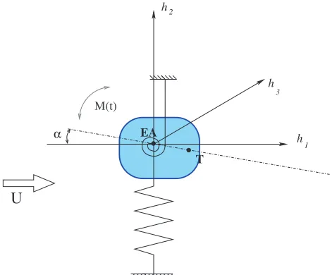
Fig. 1. A model problem of a solid body immersed in fluid is
considered, whose motion allowing torsionαand displacement
hin three directions is driven by the aerodynamical forces.
Jacobian
J(x,t)=Jˆ(ξ,t)=detDA
Dξ(ξ,t)>0,wherex=At(ξ).
and the domain velocitywD:M →Rdefined
ˆ
wD(ξ,t)=wD(A(ξ,t),t)= ∂A
∂t (ξ,t) ∀ξ∈Ω0. The Navier-Stokes equations (1) can be equivalently written either in the non-conservative formulation
DAui
Dt +(u−wD)·∇ui−2ν ∂Si j
∂xj +
∂p ∂xi =
0,∇·u=0. (3)
or in the ALE conservative way
1 J
DA Dt
Jui
+∇·((u−wD)ui)−2ν
∂Si j
∂xj+
∂p
∂xi =0,∇·u=0.
(4)
Structure motion. In this paper, the solid body which can be displaced byh=h(t)∈R3. For the sake of brevity, only the rotation around the elastic axis (EA) placed at the center of gravity (CoG) parallel toz-axis is allowed by the angleα=α(t). The equation of motion reads
mh¨ +Kh=F(t), (5) Iα¨+kαα=M3(t).
wheremis the mass of the airfoil,Iαis the moment of in-ertia around the (EA). The diagonal matrixKdenote the stiffness coefficients. On the right-hand side the aerody-namical forceF(t) and the aerodynamical momentM3(t) are involved given by
Fi=
ΓWt
σi jnjdS, M =
ΓWt
ε3i jriσjknkdS, (6)
whereεmikis the Levi-Civita symbol,r=(r1,r2,r3) and
σi j=ρ
−pδi j+2νSi j
,r=x−xCG, (7)
andxCGis the position of the CoG at the time instanttand nis the unit outward normal to∂Ωt. Let us mention, that
this is only a model problem, used to derive the variational weak form of the problem and show, that a basic energy estimate can be well estabilished in this case. However, almost the same approach can be used for more relevant technical applications as motion of a solid particle driven by a fluid flow.
3 Weak formulation
For the weak formulation the function spacesQt =L2(Ωt)
andWt = H1(Ωt) are employed for the pressure and the
velocity, respectively, defined at anyt∈ (0,T). The space for test functions is defined by
Xt={ϕ∈H1(Ωt) : ϕ|ΓD∪ΓWt=0}.
Flow problem. The weak formulation of the Navier-Stokes equations reads: FindU = (u,p) ∈ Wt×Qt such thatu
approximately satisfy boundary conditions (2) and
d dt
u,z Ωt
+νS(u),S(z)
Ωt
+c(u−wD;u,z)
(8) −p,∇ ·z
Ωt − 1
2((∇ ·wD)z,u)Ωt+
∇ ·u,q
Ωt =0
holds for allV=(z,q),q∈ ×Qt, wherez(At(ξ),t)=zˆ(ξ),
ξ∈Ω0zˆ∈X0, and
c(w;u,z)=
Ωt 1
2((w· ∇)u)·z− 1
2((w· ∇)z)·udx
+1 2
ΓO
(w·n)+u·zdS,
and where by (·,·)Gthe dot-product inL2(G) is denoted. Similarly, the weak formulation of ALE non-conservative equations (3) read: FindU=(u,p)∈Wt×Qtsuch thatu
approximately satisfy boundary conditions (2a,b) and
DAu
Dt ,z
Ωt
+νS(u),S(z)
Ωt
+c(u−wD,u,z)
(9) −p,∇ ·z
Ωt +1
2((∇ ·wD)z,u)Ωt+
∇ ·u,q
Ωt =0
holds for allV =(z,q)∈Xt×Qt. It should be noted, that
both the formulations (8) and (9) are formally equivalent.
Aerodynamical forces. In order to formulate the aero-dynamical forcesF weakly, we shall use a functionϕ ∈ H1(Ω
t) such thatϕ(x,t)= 1 for x∈ΓWt, and its compact
of (3) by the functionΨk,h = (Ψik,h), whereΨik,h(x,t) = δikϕ(x,t),k=1,2,3 integrating overΩt, applying Green’s
theorem to viscous and pressure terms, using the notation w=u−wD, we get
DAu
Dt +(w· ∇)u,Ψ
k,h
Ωt
+νS(u),S(Ψk,h)
Ωt −p,∇ ·Ψk,h
Ωt +
ΓWt 1
ρ(σi,jnj)·Ψik,hdS =0
Thus with the aid of (6), and havingΨik,h =δikonΓWt, we
get the weak form of the components of the aerodynamical forceF:
Fk=−ρ
Ωt
DAu
Dt ·Ψ
k,h+((w· ∇)u)·Ψk,h
(10) −p(∇ ·Ψk,h)+νS(u) :S(Ψk,h)dx.
Similarly, with the vector-valued functionΨα = (Ψiα) = (ϕε3ikrk), we get
ρ
Ωt DAu
Dt ·Ψ
m,α+((w· ∇)u)·Ψm,α−p(∇ ·Ψm,α)
+νS(u) :S(Ψm,α) dx+
ΓWt 1
ρ(σi,jnj)·Ψim,αdS =0,
where (σi,jnj)·Ψiα=ε3ikσi,jnjrkonΓWt, and thus
M =−ρ
Ωt
DAu
Dt ·Ψ
m,α+((w· ∇)u)·Ψm,α
(11) −p(∇ ·Ψm,α)+νS(u) :S(Ψm,α)dx.
Structure displacement and grid velocity.A pointξ∈ ΓW0from the airfoil surface is at time instantttransformed to the pointx(t)∈ΓWtgiven by
x(t)=ξCoG+h+Rα(ξ−ξCoG) (12)
whereξCoG denotes the location of the CoG in the
refer-ence domain (i.e. at the timet= 0). Now, with the aid of the previously defined functionsΨi,h andΨα, the domain
velocitywDon the surface of the airfoilΓWt satisfies the
relation
wD(x,t)=hΨ˙ h(x,t)+α˙Ψα(x,t) (13)
for anyx∈ΓWt andt ∈[0,T]. Without loss of generality
we can assume that the functionΨh,i(x,t),Ψα(x,t) are cho-sen such that equation (13) holds for anyx∈Ωt. Further,
we multiply equation (10) by ˙h, multiply equation (11) by ˙
α, sum them, and get
˙
h·F +αM˙ =−ρ
Ωt DAu
Dt +(w· ∇)u
·wD
(14) −p(∇ ·wD)+νS(u) :S(wD) dx.
Substituting for L and M from equations (5) to the left-hand side of equation (14) leads to
˙
hL+α˙M= d dt
1 2mh˙
2+1 2Iαα˙
2
+ d dt
1
2Kh·h+ 1 2kαα
2
(15) Further, the right hand side of the equation (14) has a sim-ilar form to the (non-conservative) ALE weak formulation (9), if we take the test function z = wD = h˙Ψh(x,t)+
˙
αΨα(x,t). In order to get an energy estimate for solution of (9), we continue only with a simplified problem.
Energy estimate for the simplified model. Assuming now, thatuD ≡ 0 and ΓO = ∅, we write the solutionu
as u = (u−wD)+ wD, where the first part z = (u−
wD) ∈ Xt, and where for the last term we already found
the identity (14). Now, ifuD≡0, then an apriori estimate
for the simplified coupled problem can be derived in the form
0= d dt
Ωt 1 2ρ|u|
2dx+νρ
Ωt
S(u) :S(u) dx
(16) +d
dt 1
2Kh·h+ 1 2kαα
2
+ d dt
1 2mh˙
2+1 2Iαα˙
2
,
which is the energy estimate consisting of the sum of the fluid kinetic energy, the dissipation term, the structural po-tential energy and the structural kinetic energy, respectively.
4 Numerical approximation
Time discretization For the sake of simplicity, we con-sider the equidistant partitiontk =kΔtof the time interval
I with a time stepΔt > 0, and denote the approximations uk ≈ u(·,t
k) and pk ≈ p(·,tk). Moreover we approximate
the domain velocity wD at time leveltkby wkD.
Further-more, in what follows only the non-conservative ALE for-mulation shall be used, although in ALE frame the conser-vative ALE formulation can have an influence on the qual-ity of the numerical solution. Let us focus on the descrip-tion of the discretizadescrip-tion at an arbitrary time stept=tn+1, which is kept fixed in this section (for the sake of simplicity we shall omit the subscriptstandtn+1). We shall consider all the function spacesX,W,Qdefined for this time in-stant t = tn+1 on the domain Ω := Ωtn+1. Then the time derivative in the weak formulation (8) is approximated at the timet =tn+1by the second order backward difference formula, i.e.
DAu Dt ≈
3un+1−4 ˜un+un−1
2Δt ,
where ˜uk=uk◦ Atk ◦ A− 1
tn+1. Using this, we define
a(U∗,U,V)=
3
2Δtu,z
Ω+(νS(u),S(z))Ω+(∇ ·u,q)Ω +c(u∗−wn+1
D ;u,z)−
p,∇ ·z Ω+
1 2
(∇ ·wn+1
D )u,z
Ω
L(V)= 4 ˜u
n−u˜n−1 2Δt ,z
whereU = (u,p),V = (z,q),U∗ = (u∗,p). Weak ALE formulation of the time discretized problem reads: Find U= (un+1,pn+1)∈W ×Qsuch that for all test functions V=(z,q) whereq∈Qandz∈Xholds
a(U,U,V)=L(V). (17)
D
C
B A
ξ
ξ ξ
1
2 3
A
C B
D E
F G
H
2 3
1
ξ
ξ ξ
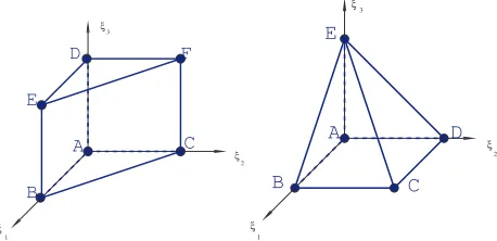
Fig. 2. The reference tetrahedral and hexahedral elements.
A
F
E D
C
B
1
2 3
ξ
ξ ξ
A
C B
D E
1
2 3
ξ
ξ ξ
Fig. 3. The reference prism and pyramidal elements.
Finite element spaces Further, the solutionuandpis sought on a couple of the finite element spaces WΔ ⊂ H1(Ωn+1) and Q
Δ ⊂ L2(Ωn+1) for the approximation of the velocity components and the pressure. The finite ele-ment spacesWΔ, XΔ, QΔ are defined over an admissible triangulationTΔof the domainΩ, cf. [20], formed by a fi-nite number of closed elementsK∈ TΔwith the following properties:
A1 Ω=K∈TΔK,
A2 The intersection of two different elementsK,K∈ TΔ is either empty or a common edge or a common vertex or a common (triangular or quadrilateral) face of these elements,
A3 K ∈ TΔis either tetrahedron, hexahedron, pyramid or prism, see figures 2-3.
Further, on the reference tetrahedral and hexahedral ele-ments ˆKwe definePK as piecewise linear functionsPK =
P1(K) and piecewise trilinear functionsPK = Q1(K), re-spectively. For the prism reference element the spacePKis
chosen as linear functions in the reference variablesξ1, ξ2 and bi-linear inξ1,ξ3andξ2,ξ3. The definition ofPKon the
pyramidal element is slightly more complicated, see [21], but the definition allows the linearity of the shape func-tions on each face, which makes the finite element space consistent.
The finite element spaces are defined by
QΔ=
ϕ∈C(Ω) : ϕK∈PK,∀K∈ TΔ
, WΔ=[QΔ]3.
By XΔ ⊂ WΔ the subspace of the test functions is de-noted. The introduced finite element spaces do not sat-isfy the Babuˇska–Brezzi (BB) inf-sup condition [see, e.g., [22], [23] or [24]], and the problem requires to use a sta-bilization, here based on the pressure stabilizing/ Petrov-Galerkin method (PSPG), see, e.g., [25].
Stabilized problem In order to stabilize the method the fully stabilized scheme is used, which consists of streamline– upwind/Petrov–Galerkin(SUPG) and PSPG stabilization com-bined with the div-div stabilization, cf. [25]. The stabilized discrete problem reads: FindU=(un+1
Δ ,pnΔ+1)∈WΔ×QΔ such thatun+1satisfies approximately the Dirichlet bound-ary conditions (2,a,b) and
a(U;U,V)+L(U;U,V)+P(U,V)=L(V)+F(V), (18)
holds for allV =(z,q)∈XΔ×QΔ, where the termsLand F are the SUPG/PSPG terms defined by
L(U∗,U,V)=
K∈TΔ
δK
Ra K(w
n+1
;u,p),wn+1· ∇z+∇q
K,
(19) F(V)=
K∈TΔ
δK
Rf K,
wn+1· ∇z+∇q
K,
where the functionwn+1=u∗−wnD+1stands for the trans-port velocity, and the terms Ra
K andR f
K are parts of the
local residual defined by
Ra
K(v;u,p)=
3u
2Δt −νu+(v· ∇)u+∇p, (20) Rf
K =
1 2Δt(4 ˜u
n−u˜n−1).
The div-div stabilizing termsP(U,V) read
P(U,V)=
K∈TΔ
τK(∇ ·u,∇ ·z)K. (21)
Here, the choice of the parameters δK andτK is
car-ried out according to [25] or [26] on the basis of the local element lengthhK, i.e.
τK =ν·
⎛
⎜⎜⎜⎜⎝1+Reloc+ h
2
K
ν·Δt
⎞
⎟⎟⎟⎟⎠, δK=
h2
K
τK,
(22)
where the local Reynolds numberRelocis defined as
Reloc= hKvK
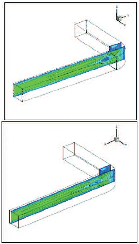
Fig. 4. The geometry of 3D domain with pressure contours.
5 Numerical results and conclusion
Numerical results The finite element method was im-plemented by an in-house software, and applied for so-lution of flow in bent channels shown in figure 4. The comparison of the results obtained by the presented finite-element method to the finite volume method is shown in figures 5 and 6 for the flow in bent channels with 90 or 180 degrees. The Reynolds number for the considered case was chosen asRe=600. For the bent channel with 90 de-grees, the separation zone appears close to the bent part of the boundary. Both the methods predicted similar structure of the separation zones. For the finite volume code, struc-tured multiblock hexahedral mesh was used with approxi-mately 60000 cells, for the finite element the unstructured hexahedral mesh was used with either 60000 or 120000 elements (without significant differences). For both meth-ods, the mesh was refined nearby the boundary to capture the boundary layer. The results shows very good agree-ment of both methods, see figure 5. Similarly, the flow in the bent channel with 180 degrees was approximated, where slightly higher number of elements were used (ap-proximately 70000 both for finite volume and finite elment cases). Both methods leads to very similar results, see fig-ure 6.
Conclusion The presented paper is devoted to two top-ics, the first one is the variational formulation of a prob-lem of a solid body immersed in flowing fluid, where the problem was thouroughly analyzed and an a priori energy estimate was shown under simplifying assumptions. Let us mention, that this estimate can be very important for numerical approximation espesically in the case of fluid-structure interactions [27] or motion of particles immersed in fluid driven by its flow. Let us mention, that the estimates shown here are the base for the estimates required for the
Fig. 5. FEM in 3D - verification, bent channel 90 degree, Re=
600, FEM to FVM comparison.
discrete solution, for the discrete problem in 2D the prob-lem was analyzed in [27], [28]. This situation is however much more complicated for 3D.
Furthermore, the finite element method was used for approximation of 3D flow in two channels and the results were verified by comparison with numerical results of fi-nite volume method. The solution by fifi-nite element method is based on the solution of the coupled problem both for ve-locity and pressure unknowns. On the other hand, for the fi-nite volume method is based on the artificial compressibil-ity method and the viscous terms are reconstructed from dual volumes. As the underlying numerical methods dif-fers significantly, the presented results can serve as a veri-fication of the results.
Fig. 6. FEM in 3D - verification, bent channel 180 degree, Re= 600, FEM to FVM comparison.
References
1. M. Paidoussis, Fluid-Structure Interactions. Slender structures and axial flow(Academic Press, Elsevier, 2013), 2nd Edition
2. T. Sucipto, M. Berci, J. Krier, Com-puters and Structures p. 15 pp. (2013), http://dx.doi.org/10.1016/j.compstruc.2013.03.004 3. P. Louda, P. Sv´aˇcek, J. Foˇrt, J. F¨urst, J. Halama,
K. Kozel, Applied Mathematics and Computation219, 7206 (2013), ESCO 2010 Conference in Pilsen, June 21- 25, 2010
4. S. Mabuza, D. Kuzmin, S. ˇCani`c, M. Bukaˇc, Journal of Computational Physics276, 563 (2014)
5. A. Hellsten, AIAA Journal43, 1857 (2005)
6. T. Bodn´ar, J. Pˇr´ıhoda, Flow Turbulence Combust76, 429 (2006), doi: 10.1007/s10494-006-9030-x
7. P. Sv´aˇcek, P. Louda, K. Kozel, Journal of Computa-tional and Applied Mathematics270, 451 (2014)
8. M. Berci, P.H. Gaskell, R. Hewson, V. Toropov, J Flu-ids Struct38, 3 (2013)
9. T. Bodn´ar, G.P. Galdi, v. Neˇcasov´a, eds., Fluid-Structure Interaction and Biomedical Applications (Birkh¨auser Basel, 2014)
10. K.J. Bathe, ed., Computational Fluid and Solid Me-chanics 2011, Vol. 89 (Elsevier, 2011), proceedings Sixth MIT Conference on Computational Fluid and Solid Mechanics
11. K.J. Bathe, ed., Computational Fluid and Solid Me-chanics 2013. Proceedings Seventh{MIT}Conference on Computational Fluid and Solid Mechanics, Vol. 122 (Elsevier, 2013)
12. S. Basting, M. Weismann, Journal of Computational Physics255, 228 (2013)
13. W. Boscheri, M. Dumbser, Communications in Com-putational Physics14, 1174 (2013)
14. M. Braack, P.B. Mucha, Journal of Computational Mathematics32, 507 (2014)
15. C.H. Bruneau, P. Fabrie, International Journal for Nu-merical Methods in Fluids19, 693 (1994)
16. J.G. Heywood, R. Rannacher, S. Turek, Int. J. Numer. Math. Fluids22, 325 (1992)
17. P. Louda, J. Pˇr´ıhoda, K. Kozel, P. Sv´aˇcek, International Journal of Heat and Fluid Flow43, 268 (2013) 18. D.C. Wilcox, Turbulence Modeling for CFD (DCW
Industries, 1993)
19. F. Nobile, Ph.D. thesis, Ecole Polytechnique Federale de Lausanne (2001)
20. P.G. Ciarlet,The Finite Element Methods for Elliptic Problems(North-Holland Publishing, 1979)
21. C. Wieners, Preprint, University of Stuttgart (1997) 22. V. Girault, P.A. Raviart, Finite Element Methods for
the Navier-Stokes Equations(Springer, Berlin, 1986) 23. P.M. Gresho, R.L. Sani,Incompressible Flow and the
Finite Element Method (John Wiley & Sons, Chich-ester, 1998)
24. R. Verf¨urth, R.A.I.R.O. Analyse num´erique/ Numeri-cal analysis18, 175 (1984)
25. T. Gelhard, G. Lube, M.A. Olshanskii, J.H. Starcke, Journal of Computational and Applied Mathematics 177, 243 (2005)
26. P. Sv´aˇcek, M. Feistauer, Application of a Stabilized FEM to Problems of Aeroelasticity, in Numerical Mathematics and Advanced Application (Springer, Berlin, 2004), pp. 796–805, ISBN 3-540-21460-7 27. P. Sv´aˇcek,Numerical Simulation of Aeroelastic
Prob-lems with Consideration of Nonlinear Effects, in Top-ical Problems of Fluid Mechanics 2008(Institute of Thermomechanics CAS, Praha, 2008), pp. 105–108, ISBN 978-80-87012-09-3