International Journal of Innovative Research in Science, Engineering and Technology
An ISO 3297: 2007 Certified Organization Volume 6, Special Issue 4, March 2017
National Conference on Technological Advancements in Civil and Mechanical Engineering – (NCTACME'17)
17th -18th March 2017
Organized by
C. H. Mohammed Koya
KMEA Engineering College, Kerala- 683561, India
Comparative Study of LES and RANS
Simulation of a Flow across a Backward
Facing Step
Arun G Nair1, Tide P. S.2, Gireeshkumaran Thampi B. S.3
Assistant Professor, Department of Mechanical Engineering, Universal Engineering College, Thrissur, Kerala,India1
Professor, Department of Mechanical Engineering, School of Engineering, CUSAT, Thrissur, Kerala,India 2
Associate Professor, Department of Mechanical Engineering, School of Engineering, CUSAT, Thrissur, Kerala,India 3
ABSTRACT: A computational procedure of significant accuracy and generality is required to predict the ambiguity
related to the turbulent flows. In this study flow across a backward facing step was modelled and analysed. The flow is analysed using two flow models in order to compare their predictive capability. The flow models used were Reynolds Averaged Navier Stokes (RANS) equation model of turbulence and Large Eddy Simulation (LES) flow model. The results thus obtained were compared with that of the experiment. It was seen that the results obtained by LES model bear close resemblance with the experimental results. Though RANS model was able to predict the first recirculation zone, it was unable to predict the second recirculation zone near the bottom wall. But LES model was able to capture the recirculation zones near top and bottom walls. The LES model is found to have a better predictive capability regarding the fluid flow problems than RANS model.
KEYWORDS: Large Eddy Simulation, Reynolds Averaged Navier Stokes Equation, Backward facing step.
I.INTRODUCTION
(Computational Fluid Dynamics) is one such viable tool to discover the physics behind turbulence. CFD is having a wide area of application. It can be used to model simple flows like two-dimensional jets, wakes, pipe flows and more complicated three dimensional ones even inside the combustion chamber that may include dissociation, diffusion and combustion. The main task of turbulence modelling is to develop computational procedures to predict the Reynolds stresses and the scalar transport terms with sufficient accuracy and generality. RANS model is the widespread turbulence model applied in the industrial CFD simulations. The attractive side of RANS turbulence model is that the simulation resources for reasonably accurate flow computations are modest. This approach has been in the mainstream for the past few decades. The Reynolds Averaged Naiver Stokes (RANS) computation was historically been the first possible approach. The accuracy required for the prediction of turbulent flows cannot be achieved using RANS model. In RANS model attention is focused on the mean flow, and the effect of turbulence on the mean flow properties. The averaged equations require a closure rule. Boussinesq hypothesis is the classical closure technique which was formulated in 1872. The properties predicted with RANS at a given point is a constant corresponding to the mean property value at this point. When Reynolds-averaged equations are used, the collective behaviour of all eddies must be described by a single turbulence model. However, the dependence of the largest eddies complicates the search for widely applicable models. A different approach to the computation of turbulent flows accepts that the larger eddies need to be computed for each problem with a time-dependent simulation. The universal behavior of the smaller eddies, on the other hand, should hopefully be easier to capture with a compact model. This is the essence of Large Eddy Simulation (LES) turbulence model. Large Eddy Simulation is an intermediate form of turbulent calculation which tracks the behavior of larger eddies. The method includes space filtering of RANS equation prior to computation. Post-processing of results obtained by LES throws light upon the mean flow and the statistics of resolved fluctuation whereas RANS model interprets the former alone. LES model can offer substantial advantages over RANS modeling approaches.
LES is another form of turbulence modeling which incorporates the energy of the large eddies present in the turbulent flow. The method involves space filtering of Navier Stokes equations instead of time averaging. LES is inherently three dimensional and time dependant. The computing resources for LES in terms of cost and space are large. Ferziger (1977) noted that LES need twice the computing resources than Reynolds Stress Models (RSM) for the same calculation. The filtering operation rejects the smaller unresolved eddies and resolves the larger eddies. The effect of the resolved flow and the unresolved smaller eddies are found out using a sub-grid-scale-model.
Celik et al. (2001) stated that even relatively coarser LES simulations are far better than RANS simulation as the former is able to capture the finest of the unsteadiness of the flow.
Rhea et al. (2009) compared study of RANS and LES based computation of an impinging jet orthogonally on a flat plate and validated with an experimental setup. They came into the conclusion that LES is having better predictive capacity than RANS model as the solution obtained in LES bear close resemblance with the experimental results particularly in the areas where large turbulent structures dominates.
Liu et al. (2006) conducted numerical analysis of a ribbed channel flow comparing RANS and LES. From the numerical study they captured more complex flow structures with LES. They noticed that in recirculation region RANS have poor predictive capability. LES offers good prediction of the reattachment length.
Lubcke et al. (2001) analyzed turbulent flow across the bluff body with RANS and LES models. An advanced RANS model, Explicit Algebraic Stress model (EASM) was used. EASM did not predict the flow properties accurately compared to that of experimental results. But values predicted with LES gave reasonable agreement with the experimental results. However EASM required very less computation time compared to LES.
Comparison of RANS and LES was done by Caciolo et al. (2011) in the context of natural ventilation in buildings. They compared RANS and LES models with the experiments results. The ventilation airflow rates computed by LES bears close resemblance with the experimental results than RANS as the former was able to capture the characteristics of the turbulent flow. However the computation time for LES was about 30 times when compared with RANS.
Prediction of turbulent flows in a stage of an axial compressor using LES was done by Nicolas Gourdain (2013). He compared the results with URANS and with experiments. This study confirms that LES predicts the time dependent flow parameters accurately than URANS near the casing.
Waarzecha and Bojuslawski (2013) modeled the pulverized coal burner in swirl chamber using LES and RANS for turbulent flow. In RANS model there exists two temperature zones-a cold and a hot zone- which is separated by the fresh incoming air into the combustor. Such a partition in the combustion chamber is not observed after computation of LES. In LES the temperature field is distributed in the chamber. With LES stronger recirculation zone was obtained compared with RANS.
II.GOVERNING EQUATIONS
The flow variables are found out by solving the differential equations.
Reynolds Averaged Navier Stokes Equation (RANS)
Reynolds Averaged Navier Stokes (RANS) turbulence model has been the widespread turbulence model used commercially and for industrial CFD. The engineers are satisfied with the computation of time averaged, flow properties like velocity, pressure, stress etc. The RANS turbulence models were therefore has been accepted worldwide. For a century these methods were widely accepted in the fields of turbulent flow calculations. The advantage that RANS model possess is that its simulation cost is less and have reasonable accuracy.
In RANS turbulence modeling, the mean or averaged flow parameter is computed. The Navier Stokes equation is being averaged with respect to time. Reynolds averaging methods were used to develop a time averaged Navier Stokes equation. The Reynolds Averaged Navier Stokes equations are given below.
During the averaging process additional terms are generated that are not in the original Navier Stokes equation. The terms are the mean of product of the fluctuations in velocity. These terms are called Reynolds stresses. A closure equation is needed in order to compute the Reynolds stresses. Such an equation was formulated in 1877 by Boussinesq who stated Reynolds stresses are proportional to the mean strain rate.
Here is called Kronecker delta whose contribution gives the correct result for the computation of Reynolds stresses.
Among the various RANS model available, k-ε model is used to compare the simulation with the experimental result. It is the most economical form of the anisotropic turbulence modeling. The k-ε model is the widespread turbulence model in industrial CFD and is the most validated model. The model is not sophisticated as it contains two transport equations. One each for turbulent kinetic energy (k) and dissipation rate (ε). This model is not compatible for swirling flows, flows along complex geometry, curved boundary layers etc.
Large Eddy Simulation (LES)
the larger eddies is to be computed. The universal characteristics of the smaller eddies are easier to model. So a single model that could accept the interaction of large eddies and the isotropic character of the smaller eddies is required to accurately predict the flow properties. Here Large Eddy Simulation comes into picture.
In LES spatial filtering is done to separate the large and the small eddies. First a cutoff width and a filter function is selected. All the eddies with the length scale greater than the cut-off width is resolved and the details regarding the smaller eddies that whose length scale is smaller than the cut-off width is destroyed. Spatial filtering is done on the time dependent governing equation. The properties of the smaller eddies and the interaction of the larger eddies with smaller eddies gives rise to the scale (SGS) stress. A model to calculate the SGS stresses is called sub-grid-scale model (SGS model). The time dependent, spatially filtered equations are solved on the grid of control volume along with the SGS model for the sub-grid-scale stresses to obtain the flow parameters and turbulent eddies of length scale larger than the cut-off width.
Spatial filtering of NS equations
The above equations are spatially filtered by means of a cut-off width (Δ) and a filtering function which is given below. As mentioned, the aim of the cut-off width and a filtering function is to separate the large and the smaller eddies.
Here, overbar indicates the filtered function. represents the filter function. Φ( ,t) is the unfiltered function. As in RANS equation the filtered function is integrated but spatially. There are various filter functions used in LES. The common filter functions are shown
Top-hat filter
Gaussian filter
γ=6
Spectral cutoff
The top hat filter is used in the finite volume methods of LES. The other two filter function is preferred by the researches.
The cut-off width is the measure of the size of eddies that are retained in the flow. The cut-off width can be of any size. Usually the cut-off width will be of the order of the grid size because it is meaningless to take a cut-off width less than the grid size. And if a greater cut-off width is used some finer details will be lost. The cut-off width is equal to the cube root of the volume of the grid cell.
as Δx, Δy and Δz represents the dimensions of the grid.
The first term represents the rate of change of filtered momentum in x, y and z coordinates. Second term represents the convective and forth term shows the diffusive fluxes. Third term gives the pressure gradient. The last term is caused due to the spatial filtering of the equations. They can be considered as the divergence of stresses.
The stresses are causes due to the interaction between the unresolved smaller eddies and these are called sub-grid-scale stresses. The SGS stresses can be calculated bu decomposition of the flow field as the sum of the filtered function with spatial variation greater than the cut-off width and are resolved in the computation and unresolved spatial variation at a length scale smaller than the cut-off width.
Using this method, the stress term can be rewritten as
Here the first term represents Leonard stress which is caused due to the filtering operation. The second term is called cross-stress. This stress term is formed due to the interaction s of the larger resolved eddies and the smaller universal eddies. The final term is called the LES Reynolds stresses caused due to the convective momentum transfer due to the interactions between the unresolved eddies. These stresses are to be modelled by means of SGS model.
Smagorinsky-Lilly SGS model
Smagorinsky (1963) suggested that Boussinesq hypothesis can give a good prediction of the unresolved eddies as the size of eddies are small and is isotropic in nature. Boussinesq hypothesis states that Reynolds stresses are proportional to mean strain rate. This hypothesis can be applied if the changes in the flow direction is slow that the production and destruction of turbulence is in a balance and eddies should be isotropic. Thus in Smagorinsky’s SGS model the local SGS stresses are taken to be proportional to the local strain rate of the resolved flow.
The proportionality constant is the dynamic SGS viscosity . is the local strain rate and is given below.
The last term in the equation ensures that the sun of the SGS stresses equals the kinetic energy of the unresolved eddies.
The Smagorinsky-Lilly SGS model is built on Prandtl’s mixing length theory which states that the SGS viscosity is related to length scale and velocity scale. The length scale in Smagorinsky model is of course the cut-off width and the velocity scale is represented as the product of cut-off width and average strain rate of resolved flow. SGS viscosity is given below
CSGS is a constant. Deardorff (1970) has done LES computation of turbulent channel flow. He addressed the value of CSGS=1 is the most appropriate for internal flow calculation and other values causes excessive damping
III. COMPUTATIONAL PROCEDURE
In this study, flow across a two dimensional backward facing step is analyzed using RANS k-ε model and LES in order to compare their predictive capability. The simulated result is then compared with the experimental results of Armaly et al. (2009). The dimensions of the backward facing step are given in figure.
The mesh was generated in ANSYS ICEM-CFD with 6,83,250 two dimensional structured quadrilateral cells. The analysis is conducted in ANSYS Fluent.
Figure 2: 2-D Structured mesh
Velocity inlet and pressure outlet boundary conditions are given at the inlet and exit of the domain respectively. The standard wall functions are used in RANS k-ε model and no-slip wall boundary condition is given to both computing methods. The SIMPLE (Semi-Implicit Method for Pressure Linked Equation) algorithm is used to calculate the pressure field. Air is the working fluid and is treated as ideal gas with constant viscosity, conductivity and specific heat.
The flow with inlet Reynolds number of 1000 is given as in the experiment conducted by Armaly et al. (1983). The flow along the backward facing step is analyzed using LES and RANS method.
Reynolds number is given by the equation given
The velocity (V) is given by two third of the maximum inlet velocity and the length (D) is twice the step thickness.
IV. RESULTS AND DISCUSSIONS
Computational study is conducted for the flow across backward facing step. Due to the occurrence of more than one recirculation zones present, the flow loses its two dimensional behaviour but as the velocity is small enough, the analysis could be conducted as a two dimensional problem.
Velocity profile at various x locations is shown in figure 3 to figure 12. It is very clear from these graphical representations that the recirculation zone exists within the flow domain. As illustrated in the figures, the prediction of these recirculation zones was done by both simulations but RANS simulation was able to capture only two recirculation zones. As the RANS turbulence model uses the averaged or mean properties to compute the results, the accuracy of the predicted result is less. In the LES model instead of mean values it takes up the filtered values using a filtering function. This allows the modelling of larger eddies with high energy and a universal model for smaller low energy eddies. In LES model more than three recirculation zones were obtained. The experimental study also imposes the same.
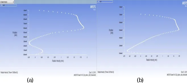
(a) (b)
Figure 3: Velocity profile at x/V2=2.55 (a) LES modelling and (b) RANS modelling
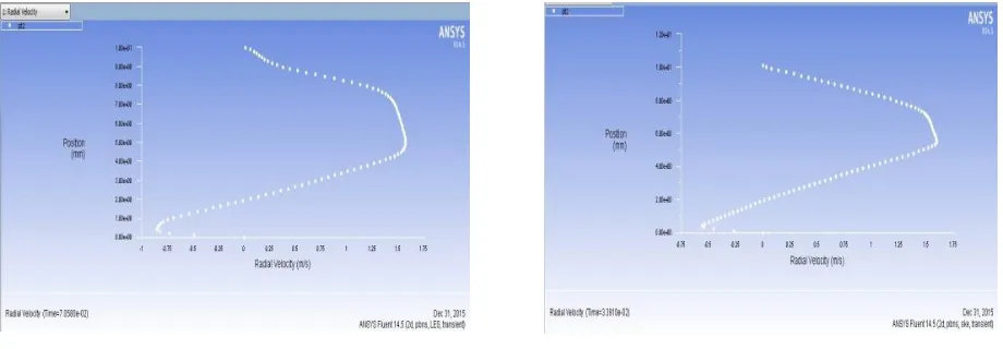
At the location x/V2 = 4, almost similar velocity profiles were obtained in both simulations. In LES simulation the recirculation zone is quite distinct as the velocity transition is almost uniform. In RANS simulation however there is a sharp change in the velocity distribution.
(a) (b)
Figure 4: Velocity profile at x/V2=4 (a) LES modelling and (b) RANS modelling
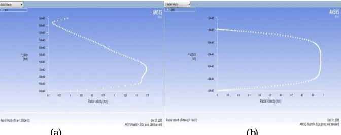
(a) (b)
Figure 5: Velocity profile at x/V2=6 (a) LES modelling and (b) RANS modelling
In figure 5 the recirculation zone is obtained in RANS simulation and the velocity is higher near the bottom wall. Beyond this location the velocity profile follows as that of fully developed flow which is a parabola with maximum velocity at its center. However the ambiguity regarding the flow is still counting. The flow dose not loses its turbulence still, according to the LES model. The second recirculation zone is being pushed further as in figure 7 and the velocity is maximum near to the bottom wall. We can see that the flow changes its direction throughout the domain showing a sinusoidal pattern till the flow becomes fully developed, as shown in figure 10
(a) (b)
(a) (b)
Figure 7: Velocity profile at x/V2=9 (a) LES modelling and (b) RANS modelling
The recirculation region near the top wall was found at location x/V2=9 using LES modelling and the flow continue to show a sinusoidal pattern as velocity is maximum near the top wall in figure 4 and it is shifted gradually to bottom wall in figure 7. The process repeats and now the maximum velocity point shifts from bottom wall to near top wall as shown in figures 8 and 9. Another recirculation point was obtained at location x/V2=12 and thereafter the flow becomes steady all along the pipe. The flow continues to be steady in RANS simulation.
(a) (b)
Figure 8: Velocity profile at x/V2=10 (a) LES modelling and (b) RANS modelling
(a) (b)
Figure 9: Velocity profile at x/V2=12 (a) LES modelling and (b) RANS modelling
(a) (b)
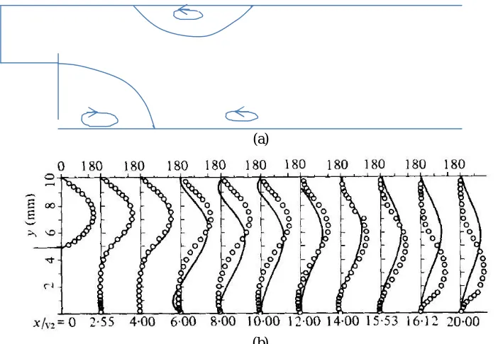
The experimental results obtained in the literature of Armaly et al. (1983) are as shown. The recirculation zones were obtained as shown. It bears a close resemblance with the LES simulation results.
(a)
(b)
Figure 14: Experimental observations (a) Recirculation zone (b) velocity profiles at various x-locations
According to the author only few velocity measurements exists for the internal flow downstream of a backward facing step. At Reynold number close to 1000, the two dimensionality of the flow is lost. Here, multiple regions of separated flow are found experimentally. The numerical results for the flow across the backward facing step are obtained as shown in figure 15.
(a) (b)
Figure 15: Velocity contour for Reynolds number of 1000 using (a) LES simulation (b) RANS simulation
V. CONCLUSION
The flow across the backward facing step using with a Reynolds number of 1000 is analyzed using Reynolds Averaged Navier Stokes (RANS) model and Large Eddy Simulation (LES) model. The turbulence model used for RANS is the k-ε model and for LES the Smagorinsky model is used.
The simulation conducted in RANS model was able to model the flow and two recirculation zones were simulated. LES model was able to capture the recirculation zones successfully.
The RANS simulations performed poorly, whereas the LES computations were again consistent and showed generally good agreement with the experiments.
The recirculation zone near the bottom wall was successfully modelled using LES but RANS model could not predict the presence the above recirculation zone. Overall, the LES turbulence models under consideration showed consistency in the flow regimes, whereas the RANS turbulence models performed poorly.
REFERENCES
[1] Yejun Gong and Franz X. Tanner, Comparison of RANS and LES Models in the Laminar Limit for a Flow Over a Backward-Facing Step Using OpenFOAM, Nineteenth International Multidimensional Engine Modeling Meeting at the SAE Congress, 2009.
[2] H K Versteeg and W Malalasekera, An Introduction to Computational Fluid Dynamics The Finite Volume Method Second Edition, Pearson Education Limited, 2007
[3] I. Celik, I. Yavuz, A. Smirnov, Large-eddy simulations of in-cylinder turbulence for internal combustion engines: a review, Int. J. Eng. Res. 2 (2) (2001) 119–148.
[5] Piotr Warzecha, Andrzej Boguslawski, Simulations of pulverized coal oxy-combustion in swirl burner using RANS and LES methods, Fuel Processing Technology 119 (2014) 130–135
[6] S. Rhea, M. Bini, M. Fairweather, W.P. Jones, RANS modelling and LES of a single-phase, impinging plane jet, Computers and Chemical Engineering 33 (2009) 1344–1353.
[7] H. Lubcke, St. Schmidt, T. Rung, F. Thiele, Comparison of LES and RANS in bluff-body flows, Journal of Wind Engineering and Industrial Aerodynamics 89 (2001) 1471–1485.
[8] Nicolas Gourdain, Prediction of the unsteady turbulent flow in an axial compressor stage. Part 1: Comparison of unsteady RANS and LES with experiments, Computers & Fluids 106 (2015) 119–129.
[9] Marcello Caciolo, Pascal Stabat, Dominique Marchio, Numerical simulation of single-sided ventilation using RANS and LES and comparison with full-scale experiments, Building and Environment 50 (2012) 202-213.
[10] B.F. Armaly, F. Durst, J.C.F. Pereira, and B. Schonung. Experimental and theoretical investigation of backward- facing step flow. J.Fluid Mech., 1983.