Hardware-Software Codesign of a Large Vocabulary Continuous Speech Recognition system.

ABSTRACT

JAYADEV, VIVEK. Hardware-Software Codesign of a Large Vocabulary Continuous Speech Recognition system. (Under the guidance of Dr Paul D Franzon).

Modern real-time applications with increasing design complexity have

revolutionized the embedded design procedure. Energy budget constraints and

shortening time to market have led designers to consider cooperative design of

hardware and software modules for a given embedded application. In

hardware-software codesign the trade offs in both the domains are carefully analyzed and

the processor intensive tasks are off-loaded to the hardware to meet the

performance criteria while the rest is implemented in software to provide the

required features and flexibility. Speech recognition systems used in real time

applications involve complex algorithms for faithful recognition. The nature of

these tasks restricts the implementation to large platforms and is not feasible to

meet the performance constraints for smaller embedded mobile systems and

battery operated devices.

This thesis proposes an idea for hardware-software codesign of a Hidden Markov

Model (HMM) based large vocabulary continuous speech recognition system.

The entire procedure can be divided into three phases: the initial phase deals

with the spectral analysis of the speech input, the second phase deals with

learning of the sound units followed by the recognition phase. Studies have

shown that the recognition phase consumes more than 50% of the processor

time. Keeping this in mind, we partitioned our design to perform the spectral

analysis and acoustic training in software using the front end executables and the

acoustic trainers provided by the CMU SPHINX. The decoder implementing the

phonetic detection and viterbi algorithm was designed in hardware. In this project

we simulated different speech input files in software and the relevant input vector

HARDWARE-SOFTWARE CODESIGN OF A LARGE VOCABULARY

CONTINUOUS SPEECH RECOGNITION SYSTEM

by

Vivek Jayadev

A thesis submitted to the Graduate Faculty of North Carolina State University

In partial fulfillment of the Requirements for the degree of

Master of Science

Electrical Engineering

Raleigh, North Carolina

2007

Approved By:

Dr. Winser E Alexander Dr. Arne A Nilsson

BIOGRAPHY

Vivek Jayadev was born on August 13th, 1982 in Bangalore, India. He received

his Bachelor’s degree in Electronics and Communications from J.S.S Academy

of Technical Education, Visveswariah Technological University, Bangalore, India

in 2004.

He joined the Master of Science program in Electrical Engineering at North

Carolina State University in August 2004. He worked under the guidance of Dr

Paul D Franzon in the area of Hardware-Software Codesign. During his graduate

program he interned with Sony Ericsson Mobile Communication, RTP, North

ACKNOWLEDGEMENTS

`

First, I would like to thank my parents and sister for their love, support and

motivation in every step of my life. I am greatly indebted to them for everything

they have done for me. Without their encouragement, I would never have been

able to succeed in my endeavors.

I sincerely thank my academic advisor Dr Paul D Franzon for giving me an

opportunity to work under his guidance. I would like to thank him for his patience

and invaluable suggestions during the course of this project. Working under him

has been a fantastic learning experience and it has given me an opportunity to

explore a variety of topics. I am very grateful to the members of my thesis

committee Dr Winser E Alexander and Dr Arne A Nilsson for devoting their time

and reviewing my thesis.

Special thanks to Dhruba Chandra for his inputs at various stages of my thesis

and making this project a success. It was a great experience working with him. I

would like to thank CMU SPHINX group for the open source recognition tools

and XILINX Inc for the design tools.

I would like to thank Ajay Babu, Deepak Kumar, Rahul Suri, Ravi Jenkal, Arun

Shashidara and all my friends for their suggestions and moral support. Finally I

would like to thank Smitha Paramshivan for being supportive and helping me

CONTENTS

List Of Tables …...………... vii

List Of Figures ………. viii

Chapter 1: Introduction ………. 1

1.1 Overview ……….. 1

1.2 Related work...……….... 1

1.3 Organization of the thesis ………. 2

Chapter 2: Speech Recognition………. ………. 4

2.1 Introduction. ……… 4

2.2 Approaches to speech recognition ………. 5

2.3 Algorithm for general speech recognition system ………. 6

2.4 Speech Recognition Softwares ……… 6

2.5 Overview of Large vocabulary continuous speech recognition ………….. 7

2.5.1 Spectral Analysis ……… 10

2.5.2 Acoustic Model ……… 11

2.5.3 Word Identification ………. 14

2.5.4 Language Model ………. 16

2.6 SPHINX speech recognition system ………... 18

2.6.1 SPHINX Executables ………. 19

Chapter 3: Coprocessor Design ………...……….. 21

3.1 Introduction ………. 21

3.2 Partitioning of Design units ………... 22

3.3 Design flow for hardware-software co-design ………... 22

3.4 Hardware-Software codesign for a LVCSR ………... 25

3.5 Hardware implementation of the Decoder ………. 27

3.6 Viterbi Algorithm ………. 29

Chapter 4: Software Implementation Of Speech Recognition………. 31

4.2 SPHINX Frontend Trainer and Decoder ………. 31

4.2.1 SPHINX Frontend………. 31

4.2.2 SPHINX Trainer…. ……….. 32

4.2.3 SPHINX Decoder………. ………... 34

4.3 Data preparation ………. 36

4.4 Tapping input vector files for hardware module ………. 37

4.5 Recognition results ……… 39

CHAPTER 5: CONCLUSION AND FUTURE WORK ……… 43

5.1 Conclusion ……….. 43

5.2 Future work ………. 44

LIST OF TABLES

Table 2-1 Monophone, Biphone and Triphone model representation………. 8

Table 2.2 Different versions of SPHINX trainers and decoders……… 18

Table 4.1: Frontend Parameters……….. 36

Table 4.2: Feature vector file ………... 38

Table 4.3: Mixture Weights file ……… 38

Table 4.4: Means file……….. 38

Table 4.5: Variance File………. 39

Table 4.6: Speech input – “ONE TWO THREE”……… 40

Table 4.7: Speech input – “R O C H E S T E R”……… 40

LIST OF FIGURES

Figure 2.1: Overview of a LVCSR……… 9

Figure 2.2: Spectral Analysis……… 10

Figure 2.3: Triphone Model……….. 11

Figure 2.4: Lexical tree structure………. 15

Figure 3.1: Design flow for hardware-software codesign……… 23

Figure 3.2: Hardware module……….. 28

CHAPTER 1

INTRODUCTION

1.1 Overview

Modern embedded systems require design optimization to realize real time

applications. Real time performance and energy budget requirements cannot be

achieved by current microprocessors. An effective solution to this problem is

hardware-software codesign. Designers using this approach, partition their

design at a very early stage to realize the timing critical part in hardware and the

rest in software.

Hardware-Software codesign is a recent area of research that focuses on

methodologies to concurrently develop hardware and software modules to meet

the cost and design constraints. The software component adds features and

flexibility, while hardware is used for performance.

This project proposes an idea for hardware-software codesign of a low power

large vocabulary speech recognition system. A general approach for most real

time speech recognizers is to start with the signal processing stage in which the

raw audio signal is spectrally analyzed and converted into acoustic vectors also

known as Mel-Frequency Cepstral Coefficients (MFCC). Then the characteristics

or parameters of the input sound units are learnt by the process of training and

this knowledge is used in deduce the most probable sound sequences.

1.2 Related work

Our project uses a HMM (Hidden Markov model) based approach [8] to

recognize the speech input files. There are quite a few software based

recognition engines successfully perform the task on large platforms but they fail

to meet the energy budget for smaller platforms like battery operated devices. In

order to meet the energy and power constraints, a hardware based coprocessor

can be used to implement the computation intensive part that occupies most of

the processor time.

We used the SPHINX open source tool provided by CMU [4] to analyze HMM

based speech recognition system on a software platform. The various front end

executables, acoustic trainers and decoders provided by the SPHINX tool were

used to process speech data and realize a complete recognition system. We

used the SPHINX 3.5 version to recognize different speech inputs whose

recognition results are presented later in chapter 4. The recognition task was

performed in a batch mode which required the input speech data to be available

before hand and prepared in the format compatible with the trainer and decoder.

The open source speech databases provided sample acoustic models,

dictionaries and test data required to implement the system.

My role in the project was to implement the software based speech recognition

process using SPHINX. The front end executables were used to convert the data

to the cepstral format compatible with the SPHINX trainer and decoder. The

feature extraction of the speech input that were spoken using a microphone were

performed using audio translation tools and the “wave2feat” executable provided

by CMU [4]. The acoustic models were successfully trained using the speech

inputs that were manually recorded. These self trained acoustic models were

used by the SPHINX decoder to recognize the spoken inputs. Good recognition

results were achieved using self trained models. Other speech databases like the

AN4 (alphanumeric) small vocabulary database [33] and HUB4 database were

used to compare recognition results. After realizing the entire recognition system

in software, the input parameter files required by the hardware module [2] were

tapped for analysis. The input files were simulated with the hardware module

The decoder performing the recognition task involved the computation of the

observation probability and used Viterbi decoder [1] to determine the most

probable word sequences. This procedure occupied a dominant part of the

processor time. A hardware module performing this task was designed in verilog

[2] and the software routine performing this function was identified in the software

decoder source code and the relevant input parameter files were tapped for

hardware analysis.

1.3 Organization of the thesis

Chapter 2 gives an overview of different speech recognition techniques and an

elaborate description of Hidden Markov model (HMM) based speech recognition

for a large vocabulary continuous speech recognizer. Chapter 3 describes the

purpose of hardware-software codesign and an overview of the hardware module

that performs the computation intensive task in the decoder. Chapter 4 deals with

the speech recognition on a software platform using the SPHINX system and

some of the recognition results using the self trained acoustic models and

existing models from the speech databases. Finally Chapter 5 has a brief

CHAPTER 2

SPEECH RECOGNITION

2.1 Introduction

Speech recognition is the process of automatic extraction or determination of

linguistic information conveyed by speech using a computer or other electronic

devices. It is a process by which a computer maps an acoustic speech signal to

text. Recognizing speech and visual features are important applications for future

embedded mobile systems. Real time scenarios demand high performance and

accuracy, which involve complex algorithms as illustrated in the following

chapters.

A speech recognition system can be characterized by many parameters based

on their ability to recognize speech. Some general classification:

• Speaking Mode: Recognition systems can be either isolated word processors

or continuous speech processors. Some system process isolated utterances

which may include single word or even sentences and others process

continuous speech in which continuously uttered speech is recognized that is

implemented in most real time applications.

• Speaking Style: A speech recognizer can either be speaker-dependent or

speaker-independent. For speaker-dependent recognition, the speaker trains

the system to recognize his/her voice by speaking each of the words in the

inventory several times. In speaker-independent recognition the speech

uttered by any user can be recognized, which is more complicated process

compared to the former system.

• Vocabulary: The size of vocabulary of a speech recognition system affects

the complexity, processing requirements and the accuracy of the system. A

medium vocabulary system can extend to 1000 words (RM1) and a large

vocabulary system can extend to approximately 64,000 words (HUB4) [7]

2.2 Approaches to Speech Recognition

Some of the modern recognition techniques which are commonly used are:

•

Hidden Markov model (HMM) based speech recognition [8]: Modern

recognition procedure emphasize on HMM based recognition, which

has a rich mathematical structure to provide accurate results for a

typical large vocabulary continuous recognition systems. This

approach is popular because of the precise mathematical framework,

the ease and availability of training algorithms for estimating

parameters of the models from finite training sets of speech data. An

added advantage is the flexibility of the resulting system where one

can easily change the size or architecture of the models to suit the

user’s requirements. A HMM can be used to reduce a non-stationary

process to a piecewise-stationary process. Speech could be assumed as

short-time stationary signal for a period of 10 milliseconds and modeled as a

stationary process. Speech could thus be realized as a Markov model, which

could be trained automatically and making it computationally feasible.

• Dynamic programming approach [20]: This approach is based on dynamic

time warping (DTW) algorithm, which measure similarities between two

quantities varying with time. DTW is a template-based pattern matching

system. Each word is stored as a collection of templates. DTW stretches and

compresses various sections of the utterance so as to find the alignment that

result in the best possible match between the template and the spoken

speech signal. It turns out to be computationally intensive when operating

• Neural Network (NN) based approach [20]: This is a commonly used

approach in small vocabulary systems. The NN based approach results in

higher accuracy compared to other systems working well with dynamic

aspects of speech such as low quality data, noisy data and speaker

independence. There are also NN-HMM [NN-HMM] hybrid systems that use

the neural network part to deal with the dynamic aspects and the hidden

Markov model part for language modeling.

• Knowledge based approach: The knowledge/rule-based approach has the

acoustic, lexical or semantic knowledge about the structure and

characteristics of the speech signal explicitly stored in the system database.

The aim is to express human knowledge of speech in terms of explicit rules

like acoustic-phonetic rule, rules describing words of the dictionary, rules

describing the syntax of the language and so on. During recognition it

compares simple words with ones in the database.

2.3 Algorithm for general speech recognition system

1. Record test and training data for detection

2. Pre-Filtering (pre-emphasis, normalization) and spectral analysis

3. Framing and Windowing (Front end)

4. Learn the characteristics of the speech input (training)

5. Comparison and Matching (recognizing the utterance)

6. Action (Perform function associated with the recognized pattern)

2.4 Speech Recognition Softwares

Based on the different approaches to speech recognition there are a number of

software tools available in the market for its implementation. We used the Hidden

Markov model based SPHINX open source tools developed by CMU [4] which

includes trainers, decoders, acoustic models and language models required to

build a complete speech recognition system. Other softwares which use HMM

Speech Vision and Robotics Group at the Cambridge University, Audio-visual

continuous speech recognition (AVCSR) using coupled Hidden Markov Models

[28], Internet-Accessible Speech Recognition Technology (ISIP) [27] and Dragon

recognition systems introduced by Baker using Hidden Markov models [29].

Neural network based speech recognition can be implemented in the software

domain using tools like the NICO tool kit [31] and Quicknet tool from the

SPRACHcore package [32]. There are hybrid recognition tools combining both

the HMM and neural network techniques also available in the market. The

dynamic programming approach to recognition can be realized using Jialong

He's Speech Recognition Research Tool [30].

2.5 Overview of Large vocabulary continuous speech recognition

(LVCSR):

We used a HMM based approach [37] to perform the speech recognition task in

our project. Due to large vocabularies in the real world, it is practical to design

acoustic models at a phonetic level. The basic sounds that represent all the

words in the vocabulary are called as phones or phonemes. There are

approximately 50 phones that can be used to define all the words in the English

dictionary. A straightforward approach is to encode words to represent them in

terms of phones. These kinds of models which do not take the context into

consideration are called context-independent or monophones. However phones

are not produced independently, it is strongly affected by the mechanical limits of

speech sound production leading to co-articulation effects. In order to overcome

these disadvantages, a context dependent model called biphone or triphone

model that takes into consideration the immediate left and the right neighboring

phones is used. So every phone has a distinct HMM model for every unique pair

of left and right neighbors. The word “AUGUST” can be represented in different

Table 2-1: Monophone, Biphone and Triphone model representation.

Monophone Model SIL AA G AH S T SIL

Biphone Model SIL-AA AA-G G-AH AH-S S-T T-SIL

Triphone Model SIL-AA+G AA-G+AH G-AH+S AH-S+T S-T+SIL

The context independent models or the monophone model is represented in

terms of individual phones. The models can include SIL which is a special phone

that denotes silence and can also include breath pauses. The interaction

between phonological rules, speech impairment and coarticulation affect are

taken into consideration while building the context dependent models like the

biphone and triphone models. Biphone models consider either the left context or

the right context phone. For the triphone example illustrated in table 2-1 the first

and the last triphones are SIL-AA-G and S-T-SIL respectively which are of the

format left_context - current_phone + right_context. There are approximately

50x50x50 = 125,000 triphones possible, of which only 60,000 are considered in

English. Context-dependent systems always perform better (in terms of word

error rate) than a context-independent system. Now the probability that an

acoustic vector corresponds to a triphone is determined using the Hidden Markov

Model. The exit of one state in a triphone is merged to an entry state of another

triphone forming a composite HMM. [3][16][17]

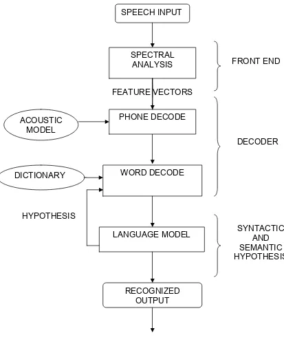
The different steps in continuous speech recognition system are illustrated in the

Figure 2.1: Overview of a LVCSR. SPECTRAL

ANALYSIS

PHONE DECODE

WORD DECODE SPEECH INPUT

LANGUAGE MODEL

RECOGNIZED OUTPUT ACOUSTIC

MODEL

DICTIONARY

FEATURE VECTORS

FRONT END

DECODER

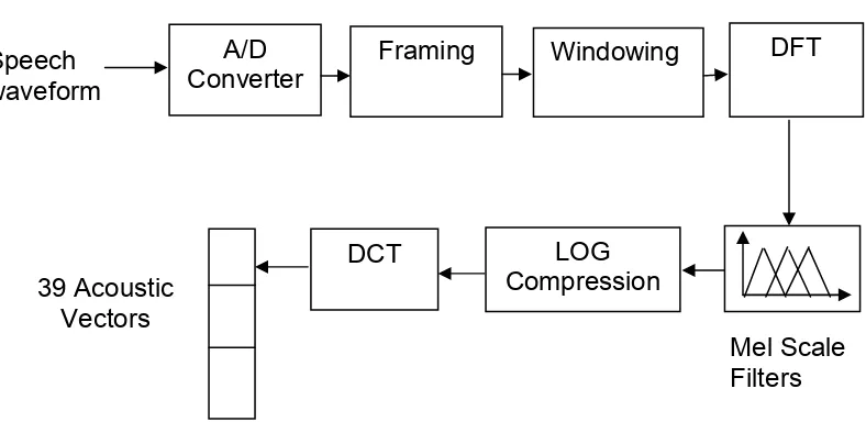
2.5.1 Spectral Analysis

Each word is assumed to be composed of a sequence of basic sounds called

phones or phonemes which is represented by a HMM. Any spoken input to the

recognizer has to be parameterized into a discrete sequence of acoustic vectors

(MFCC)[10] in order to represent its characteristics using a Hidden Markov

model. This process is called spectral analysis and is implemented as shown in

figure 2.2.

Figure 2.2: Spectral Analysis.

The speech signal is considered to be stationary over a small interval of time

typically 10msecs. This helps the signal to be divided into blocks and from each

block a spectral estimate is derived. The blocks are normally overlapped to give

longer analysis window of approximately 25msecs, which reduces signal

discontinuity.

The analog speech waveform is band limited using a low pass filter and

converted into a digital signal using an A/D converter. The signal is then

premphasized to compensate for any attenuation caused. A windowing function A/D

Converter Speech

waveform

Framing Windowing DFT

LOG Compression DCT

39 Acoustic Vectors

is usually applied to minimize the effect of discontinuities. The signal is then

converted to the frequency domain using the Fourier transform. To represent the

auditory characteristics more precisely to human hearing system at different

frequencies a set of overlapping triangular Mel-scale filters is used. The range of

values generated from the non-linear Mel-scale filters are reduced using log

compression.

The Discrete cosine transform (DCT) is used to compress the spectral

information into a set of lower order coefficients, which is called Mel-Frequency

Cepstral Coefficients (MFCC). The MFCC obtained from DCT is generally

appended with time derivatives to overcome the decorrelation with the

predecessors and successors.

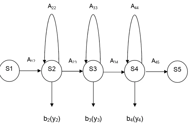
2.5.2 Acoustic Model:

Figure 2.3: Triphone Model

Each basic sound in the recognizer is modeled by a HMM as shown in figure 2.3.

It consists of a sequence of states connected by probabilistic transitions in a

S1 S5

b2(y2)

S4 S3

S2

A44

A22

A45

A34

A33

A23

A12

simple left-right topology. HMM phone models generally have three active states

forming a triphone model. In figure 2.3 S1 and S5 are the entry and exit states

S2, S3 and S4 are the active states. The exit state of one phone model is

merged to another to form a composite HMM.

If we consider a simple probabilistic model for speech production with W as the

sequence of specified words that are modeled and Y as the sequence of acoustic

vectors generated at the front end, the stochastic models can be used to

represent the words to be recognized [1]. The word sequence W* that has the

highest posteriori probability P(W|Y) among all possible word sequences is given

by,

W =argmax P(W|Y)

This problem can be significantly simplified by applying the Bayesian approach to

find *

W

*

w

P(Y|W)P(W)

W =argmax

P(Y)

Since P(Y) is the probability of the acoustic vectors which remains the same for

all the possible sequences it can be omitted. The equation reduces to

*

w

W =argmax P(Y|W)P(W)

In practice, only the acoustic vectors are known and the underlying word

sequence is hidden. The probability P(Y|W) is evaluated by the acoustic model

which estimates the probability of the acoustic observations. The probability of

the word sequence P(W) is evaluated using the language model [5] [2] [1]. An

n-state HMM is defined by a stochastic matrix containing the transition probabilities

of the form Aij which is the probability of transition from state Si to Sj which may

observation Y is called observation probability or the senone score. To obtain t

better accuracy by overcoming the quantization effects modern systems use

continuous probability function like multivariate Gaussian distribution [23] to

represent these observation probabilities [12]. Continuous density HMMs [10]

[11] compared to discrete or semi-continuous observation density models provide

better accuracy as the number of parameters available to model the HMM can be

adapted to the available training data. Discrete and semi-continuous models on

the other hand use a fixed number of parameters to represent observation

densities which cannot achieve high precision without using smoothing

techniques. The general representation of continuous observation density is

given by:

( )

(

)

M

,

K 1

t t

b O

C N O

µ

U

=

=

∑

Where O represents the acoustic vector being modeled, t C is the mixture jk

coefficient for the _{k mixture in state j and N is normal distribution generally} th

chosen to be a Gaussian distribution with mean vector µ (associated with state jk

j of mixture component k) and covariance matrix U (associated with state j of jk

mixture component k). The mixture gain Cjk must satisfy the constraint,

C

1

=

∑

The above equation is constrained by 1≤j ≤N and 1≤k ≤M. For a HUB-4 [36]

speech database provided by CMU M and N are defined as 8 and 39

respectively.

While working with Hidden Markov models the evaluation problem which deals

with the determination of observation sequence probability b (O ) from the given j t

observation sequence O={O ,O O1 2, 3...O }T and the speech model has been

Viterbi algorithm [1]. The main aim of Viterbi algorithm is to find the word

sequence which has the highest probability to produce the observation sequence

that could be decided by optimality criterion. The Viterbi algorithm attempts to

find the single best sequence, q={q ,q q1 2, 3...q }T for the modeled

sequenceO={O ,O O1 2, 3...O }T . This algorithm is similar to forward-backward

procedure with the only difference is the maximization over the previous states

rather than the summing procedure. Tracing back from the most probable final

state will reveal the most probable or likely state sequence. To find the single

best sequenceq={q ,q q1 2, 3...q }T the quantity δt(i) is defined by,

δ

(i)

=

max

P[q ,q ,...q

q

=

i,o o ...o | ]

λ

The quantity δt(j) gives the best score along a single path for the first t

observations. Using induction the equation 2.6 can be reduced to,

δ

( j) [max

=

δ

( )

i A ].b (O

)

From recursion the equation 2.6 can be summarized as,

δ

( j)

=

max

[

δ

( )

i A ].b (O )

Another quantity which is used to retrieve the state sequence and keeps track of

the argument maximized in equation 2.7 is given byΨt( j),

Ψ

( j)

=

arg max

[

δ

(i).A ]

The two quantities δt( j) and Ψt( j) are constrained by 2 ≤ t ≤ T and 1 ≤ j ≤ N

2.5.3 Word Identification:

A recognition system will need an exhaustive database containing the HMMs for

triphone HMMs. All the words in the dictionary are entered in the lexical tree. A

Lexical (phonetic prefix) tree is a root tree with each node representing a chain of

triphones.The search network is built using nodes that are linked to each other

using arcs. Nodes can either correspond to one HMM state or a dummy node

without any acoustic probabilities associated with them. The full triphone lexical

tree with all possible start left and end right context triphones is considered while

decoding the word. Words have more than one possible pronunciation and

therefore, multiple paths need to be explored for a given word. Words and

sentences can he constructed by concatatenating the corresponding phones that

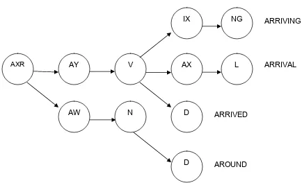
constitute their pronunciation. The lexical tree constituting four words ARRIVING,

ARRIVE, ARRIVAL and AROUND are shown in figure 2.4. The nodes are shared

if the words share the state sequence id. Each word ends at the leaf node which

remains unshared.

Figure 2.4: Lexical tree structure

AXR _{AY V AX L}

AW N D

NG IX

D

ARRIVAL ARRIVING

ARRIVED

A Common approach to a Large Vocabulary Continuous Speech Recognition

(LVCSR) system implementation is to use a lexical tree (phonetic prefix tree). A

lexical tree has words with similar pronunciation share the same starting nodes

but separate leaf nodes resulting in drastic reduction of the search space in the

LVCSR. Word identification stage uses a time-synchronous Viterbi search

algorithm to decode the lexical tree. Continuous speech can be implemented by

using null transitions from the final state of each word to the initial state of all

words. Triphones that occur at the end of a word are specially marked so that a

language model can be used to disambiguate words with similar sound.

2.5.4 Language Model

For a large vocabulary recognition system, it is not very efficient to generate a

trellis containing all the words and search for the best possible match. A

Language model assists the recognition process by taking into consideration the

various semantic and syntactic constraints. Language models require estimation

of the a priori probability P(W) of a sequence of words W = w1, w2, w3,…,wN. The

probability of a word under consideration depends on words that were previously

observed. This process of training helps the system to disambiguate words which

sound similar. The probability of the word sequence P(W) which is used in the

acoustic model to derive the highest likelihood probability to observe a sequence

of acoustic vectors is determined by the language model and can be defined for

a N-gram language model as:

Q

N 1 2, 3, ..., N i | 1, ..., i N 1

i 1

P (W)

P(w , w w

w )

P(w w

w

)

=

=

=

_∏

Estimation of such a large set of probabilities from a finite set of training data is

is chosen and the probability of P(W) depends on N -1 previous words. Thus, a

2-gram or bigram language model would compute P(w1, w2, w3, w4...) as

P(w , w , w , w ...) = P(w )P(w | w )P(w | w )P(w | w )...

Similarly, a 3-gram or trigram model would compute it as

1 2 3 4 1 2 1 3 2 1 4 3 2

P(w , w , w , w ...) = P(w )P(w | w )P(w | w , w )P(w | w , w ) ...

The value of N determines the number of probabilities to be estimated. Low

values of N are required to obtain sufficient accuracy from a limited training set.

When sufficient training data is not available for a good estimate, large values of

N produces a reduction in performance [1]. For statistical language modeling of

N-gram language model the conditional probabilities defined in equation 2.10

PN(W)) P(wi|w1,…..,wi-N+1) can be estimated from a relative frequency approach,

i-N+1

i i-N+1

i i-1 i-N+1

i 1

F(w ,w ,...,w

)

P(w |w ,...,w

) =

F(w ,...,w

)

For a N-gram model F(wi,wi-1,…..,wi-N+1) is the frequency of occurrence of the

word strings wi,wi-1,…..,wi-N+1 in the training text. The conditional probability for a

trigram model can be defined as,

P(w3|w1,w2) =

F(w1,w2,w3)

F(w1,w2)

Where F(w1,w2,w3) is the frequency of occurrence of the trigram model and F

(w1,w2) is the frequency of occurrence of the bigram model. In a large vocabulary

continuous speech recognition system, the training database may not have all

the possible triphones so the bigram and unigram relative frequencies are

2.6 SPHINX speech recognition system

We used the SPHINX speech recognition system provided by the Carnegie

Mellon University [4] to implement the HMM based speech recognition. The

SPHINX system [19][21] is an open source tool which includes all the trainers,

decoders, acoustic models and language models required to build and test a

complete recognition system. The tools provided by SPHINX have a wide variety

of applications which cater to different needs of the user. The different versions

of SPHINX [26] along with its features are listed in table 2.2.

Table 2.2: Different versions of SPHINX trainers and decoders

VERSION FEATURES

SPHINX-2

Semi-continuous and continuous output probability

density functions.

Tree lexicon

SPHINX-3

( S3-flat )

Continuous output probability density functions.

Batch processing

Flat lexicon

LVCSR System

SPHINX - 3.X

(S3-fast)

Continuous output probability density functions.

Batch and Live mode processing

Tree Lexicon

SPHINX-4

Continuous output probability density functions.

Live mode and batch mode processing

The main advantage of SPHINX package is that it is fully customizable for a

range of different applications. The user can carefully chose the version

depending on the type of models he is working with and the level of accuracy

required.

We used SPHINX 3.5 which is a speaker independent large vocabulary speech

recognition system to perform the recognition task. The entire procedure was

realized on a LINUX/UNIX platform which has inbuilt C-compiler, Perl and audio

converter which made the task easier. The recognition was performed in a batch

mode which required the speech input to be preprocessed in a cepstral format to

be compatible with the SPHINX acoustic trainers and decoders. For a batch

mode processing the entire input that has to be recognized must be available

beforehand. The pre-recorded speech has to be processed from its raw format

into ceptrum files which is compatible with the SPHINX trainer and decoder. The

HMM based system uses the trainer to learn the characteristics of the speech

input and the decoder to deduce the most probable sequence of sound units for

a given speech input.

2.6.1 SPHINX Executables:

SPHINX trainer learns the characteristics of the sound models using a set of

programs. The training database which comprise of test data, pronunciation

dictionary, filler dictionary and the transcript files are provided to the trainer. The

trainer then functions by mapping each word to a sequence of sound units in the

dictionary and derives the sequence of sound units associated with each signal.

The trainer generates model index files which contains references to states in the

HMM models which helps both the trainer and decoder to access the right

parameters. Using the open source trainer and the relevant input files acoustic

The SPHINX decoder has a set of programs to perform the recognition task. The

input files required for the decoding procedure include trained acoustic models,

pronunciation dictionary, filler dictionary, language model and the test data in the

right format. With any given set of acoustic models, the corresponding

model-index file must be used for decoding. Both the trainer and decoder process test

data in the form of feature vectors. These feature vectors are generated from

converting the acoustic signals to a ceptsra format using the front-end executable

CHAPTER 3

COPROCESSOR DESIGN

3.1 Introduction

A coprocessor implementation is a cooperative approach used to improve the

performance by off-loading the processor intensive tasks from the primary

processor to the coprocessor. Hardware-software codesign works on a similar

approach. It is a concurrent design technique which uses the software design to

provide features and flexibility while the hardware module is used to improve the

overall system performance. Dedicated hardware modules are designed to

supplement tasks like floating point arithmetic, math operations, signal

processing and graphical applications saving a lot of the processor time.

Hardware-software codesign aims at defining the key trade off points across the

hardware and software domains. The tightly coupled hardware and software

components have predefined functions. The software component dictates the

required control functions and the ideal hardware component aims at improving

power-consumption, execution-speed and manufacturing-cost targets. The

advantages of the software components are that it’s cheaper than hardware and

it allows late design changes and simplified debugging techniques. However,

using hardware in a design becomes a necessity when the software alone cannot

meet the required performance criterion.

Hardware components are implemented using full custom hardware modules,

semi custom ASICs, FPGAs (field programmable gate arrays) or

Systems-on-chip (SOC). Systems-on-Systems-on-chip is an idea of integrating all the components of an

electronic system into a single chip. An SOC can contain digital, analog or mixed

signal functions implemented using the hardware module [25] to meet

drivers or DSP cores. The design flow for an SOC aims to develop this hardware

and software in parallel.

3.2 Partitioning of Design units

Hardware-software partitioning is a decision which is made very early in the

design procedure. Partitioning involves system level design decisions about

target architecture that decides the overall performance of the system. First a

formal model is developed to identify the different system functionalities and the

interaction between them. This will help in estimating the resources needed for

each application subtask based on design constraints in terms of cost, power

consumption, silicon size, speed, etc. Based on these constraints it assigns the

subtasks to specific target devices at compile-time, be it software or a hardware

module. Effective partitioning decisions help in reducing ambiguities during

synthesis and achieve best possible performance for the given design

constraints.

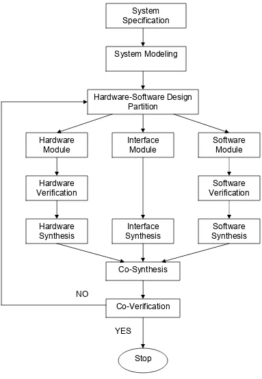
3.3 Design flow for hardware-software co-design:

The different step involved in developing an embedded system [13] involving

Figure 3.1: Design flow for hardware-software codesign System

Specification

System Modeling

Hardware-Software Design Partition

Hardware Module

Interface Module

Software Module

Hardware Verification

Software Verification

Hardware Synthesis

Software Synthesis Interface

Synthesis

Co-Synthesis

Co-Verification

Steps involved in hardware-software codesign:

• System specification and modeling: The given project specifications are

analyzed completely and broken down into application subtasks based on

the given design, cost and power constraints. This step realizes the

architecture of the target processor depending on the system

functionalities and their interaction. It specifies the behavior at the system

level which helps in design partitioning. It estimates the cost metrics for

both hardware and software modules. The software cost metrics may

include memory requirement and execution time. The hardware cost

metric deals with power consumption, execution time, chip area and

testability. Using the specifications a structural model is designed which

specifies the hardware and the software modules, a system model

illustrating the functionality and a dynamic model which represent the

transitions occurring in the system.

• Design Partitioning: Evaluating the trade-offs between the cost metrics of

the hardware and software, the designer clearly separates the functions

that are performed by each of the modules. This step plays a very

important role in resolving the problems during the co-synthesis of the

hardware and software modules. The heterogeneous target architecture

requires interface units to communicate and synchronize the hardware

and the software modules that also have to be taken into account in this

step.

• Modeling subtasks: Based on the decisions made in the design partition

stage the modules are developed in their respective platforms. This step

can be very efficient and lead to optimal results if the designer has the

flexibility to work at different levels of abstractions. There are different

tools available in the market to implement the modules at the system level

VHDL or SystemC and the software modules are designed on a C, C++ or

a JAVA platform. Interface units have to be separately designed which

play a major role in program execution and synchronization between the

modules designed in different platforms.

• Synthesis and verification: The hardware and the software modules are

individually tested and verified by algorithms and test fixtures at different

levels of abstraction. This step optimizes the design using various logic

synthesis techniques. In addition to uncovering bugs in the design it also

guides the synthesis process.

• Co-synthesis and co-verification: This co-simulation and the co-synthesis

phase concentrate on integrating both the hardware and software

modules. The resulting system is verified in the co-verification phase by

executing test case scenarios to meet the specified design constraints. If

the situation demands, the system is repartitioned again and the process

is repeated to meet the requirements. Some systems also include

co-validation that aims uncovering bugs at different abstraction levels.

Co-validation methods include formal verification, simulation or emulation.

Emulators systems map the ASICs onto programmable hardware like

FPGA (Field Programmable Gate Array) and couple them with processors

on a board.

3.4 Hardware-Software codesign for a LVCSR

Chapter 2 gives the design flow for a large vocabulary continuous speech

recognition system (LVCSR). We used a Hidden Markov model (HMM) based

approach because of the precise mathematical structure and the availability of

training algorithms to estimate the parameters of the models involved. The

that the observation is a probabilistic function of state (phonetic representation)

with an underlying stochastic process that is not directly observed but can be

determined through other set of stochastic process. The HMM based recognition

had to account for evaluating the likelihood of the sequence of observations for a

given HMM, determining the best sequence of model states and adjust the model

parameters to find the best probable observation. Real-time speech processing

requirements have performance metrics that cannot be met by current embedded

microprocessors. A solution to this problem is provided by hardware-software

codesign. The stages, which involve complex computations, can be performed by

application specific (ASICs) hardware modules improving the overall system

performance.

After evaluating the design phases involved in building a LVCSR, we separated

the modules that are implemented in software and hardware. We used the

trainers and decoders provided by CMU SPHINX [4] to perform the recognition

task. The processing can be divided into stages namely: Front end which

performs the spectral analysis and generation of the acoustic vectors, Acoustic

model which deals with multivariate Gaussian distributions to compute the

observation probabilities and lastly the language model to improve the accuracy

of recognition. Studies show that more than 50% of the processor time is used in

performing Gaussian computations to estimate the observation probabilities of

HMMs [6] for a HUB-4 speech model. This dominant phase, which mainly

involved floating point arithmetic, was realized using application specific

hardware coprocessor.

For the initial data preparation the front-end executable provided with the

SPHINX-3 training package was used to generate the data in a cepstral format.

The SPHINX-3 trainer was used to train acoustic models that were compatible

with the SPHINX-3 decoder. The tasks performed using SPHINX was in

software, which does not meet the desired performance criteria for small

part was developed in hardware [2] and coupled with the low power host

processor. All the input vectors required for the hardware modules were tapped

from the SPHINX trainer and decoder to estimate the performance results. The

Gaussian computations were done using the HUB-4 speech model and audio

databases (AN4 and RM1) provided by CMU [7].

3.5 Hardware implementation of the Decoder:

The decoder performs the recognition task, which is implemented using two

design units. The first unit computes the observation probability for all the

relevant input vector files and the second unit determines the maximum

likelihood probability using Viterbi algorithm [1] [2]. The optimal state sequence

defined in chapter two is generated by the Viterbi decoder is given by:

δ

( j)

=

max

[

δ

( )

i A ].b (O )

The best score δi (j) is defined in terms of observation probability discussed in

equation (3.1). The multivariate Gaussian distribution used to compute the

observation probability is given by

2 ji ) (Oji

2 ji

t j j

ji

1

1

N(O ,

,

)

e

2

µ σ

µ σ

π

πσ

− −

_∑

=

In the above expression Oji,

σ

The observation probability calculations involve floating point arithmetic done in

the logarithmic domain. For a HUB-4 speech model the observation probability in

2

M N

j t j _t jm t jk jk

K=1 n=1

B (O ) = log (b (O )) =

_∑

C -

_∑

[O (n) - µ (n)]

δ

(n)

The values of M and N for a HUB-4 speech model provided by CMU are chosen

as 8 and 39 respectively. The floating point computations can be made simpler

by implementing them in logarithmic domain [18] by computing the inner term

2

t jk jk

[O (n)−µ (n)] δ (n) in the data path and then using a log-add module to produce the final score. Each of the inner term can be specified as

kj jk t jk jk

A = C N(Y , µ ,U ),

log (b (O )) = log(A + A + A +...+ A )

From the expressions defined for N(O , µ , t j σj) and log(b (O )) we can deduce the j t

relation for log(A ) as, Mj

2

L

Mj jk ji ji jk

i 1

log(A )

C

(O

µ

) *

δ

=

=

−

∑

−

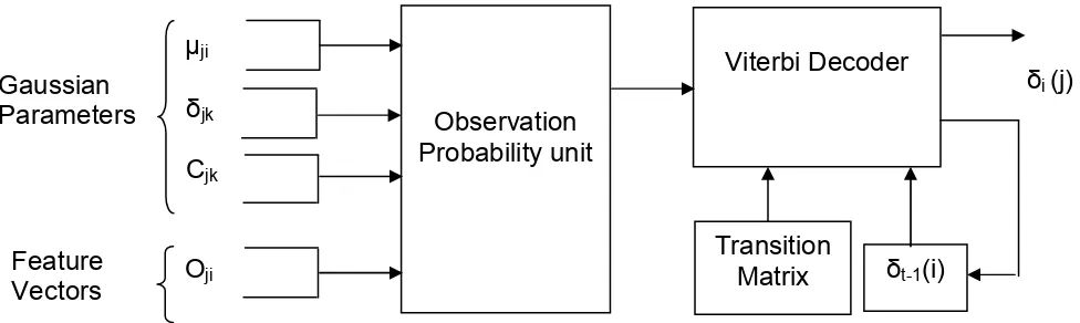
The entire hardware module with all the input parameters required to perform the

recognition task including the viterbi decoder is shown in the block diagram in

figure 3.2. The implementation of each of the hardware modules for our project is

discussed in [2].

Figure 3.2: Hardware module Observation Probability unit Cjk δjk µji Gaussian Parameters Oji Feature Vectors Viterbi Decoder

δi (j)

Transition

3.6 Viterbi Algorithm

The performance criterion for a LVCSR is decided by the design of the efficient

search algorithm which has to deal with huge search space combining the

acoustic and language models. The aim of the decoder is to determine the

highest probable word sequence given the lexicon, acoustic and language

models. The most common method adopted is the best path search through a

trellis where each node corresponds to a HMM state. Traversing the entire trellis

for the best possible path requires a lot of computing recourses which proves to

be very expensive. Using Viterbi algorithm adopts strategies like fast match,

word-dependent phonetic trees, forward-backward search, progressive search

and N-best rescoring to deal with large vocabularies.

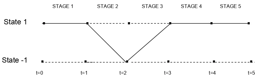
Trellis decoding [1][14] for a received sequence can be illustrated with an

example. If the received sequence is Y = (y1, y2, y3,….,yK) with each symbol

corresponding to one stage of the trellis. The viterbi algorithm computes the most

likely transition from the current state to the next state computing metrics for all

the possible paths. The example has five stages with the initial state being 1.

.

State 1

.

. . . . .

State -1

.

. . . . .

Figure 3.3: Trellis diagram for the input sequence (1, -1, 1, 1, 1)

STAGE 1 STAGE 2 STAGE 3 STAGE 4 STAGE 5

The trellis diagram is shown for the input sequence (1, -1, 1, 1, 1).The survived

path is denoted by a thick line which is the best probable path derived from

viterbi algorithm. The algorithm is very similar to the forward algorithm with the

only difference being the probabilities of transitions from all states of the previous

time step is considered and all others are discarded. The major difference is the

maximization over the previous state shown in equation 3.1 which is used

instead of the summing procedure. Tracing back from the most probable final

state gives the most probable state sequence.

In our project the viterbi algorithm is used to compute the best probable path for

the given input sequences. The Viterbi search algorithm for Hidden Markov

models is multiplication intensive which can be made simpler by realizing it in a

logarithmic domain. The mathematical equation represented in the logarithmic

domain to implement the viterbi algorithm is given in equation 3.1. The block

CHAPTER 4

Software Implementation of Speech Recognition

4.1 Introduction

This chapter gives an overview of the procedures involved in the software

implementation of the recognition process and generation of the test input files

required for the hardware module discussed in chapter 3 using SPHINX. We

used the SPHINX 3.5 (s3.5 or fast decoder) an open source tool provided by the

Carnegie Mellon University [4]. SPHINX 3.5 is a large vocabulary,

speaker-independent continuous speech recognition engine. The s3.5 is faster compared

to pervious versions and achieves better speed and accuracy on large

vocabulary tasks.

The SPHINX 3.5 provides the trainers and decoders to perform recognition for

fully continuous acoustic models. The decoders have the provision to recognize

speech in a batch mode with prerecorded speech or live speech mode from the

audio card discussed later in the chapter. The package also includes language

models, language dictionary, filler dictionary and open source speech databases

required in recognizing the given set of acoustic signals.

4.2 SPHINX Frontend, Trainer and Decoder

4.2.1 SPHINX Frontend

The speech input files that were used for the recognition were recorded using a

microphone. The audio files are generally in .wav or .au format but the SPHINX

trainer and decoders are compatible with data in cepstral format. The recorded

wave files were then converted into raw sound files which is PCM audio data

without any header information. This procedure was carried out using the “sox”

16000 Hz. The raw audio files were processed using the frontend executable –

“wave2feat” with Mel Filter bank and specified sampling rate and the endian-ness

of the audio data used. The issue of audio file processing will be dealt in section

4.3. Using the SPHINX frontend, the test and the training databases were

created. The training database was used by the trainer to generate acoustic

models and the test database was used by the decoder for the recognition task.

4.2.2 SPHINX Trainer

The SPHINX trainer provided in the package is used to train the acoustic models

and the phone model parameters. These modeled phones are used to initialize

the parameters in the actual training process. The input files including Gaussian

mean, variance, mixture weights and transition matrix required by the decoder

are produced by the trainer. For continuous speech recognition using HMMs,

explicit marking of the word boundaries is not necessary as the state sequences

are hidden. So each word can be instantiated with its model and the rest of the

words in the sentence can be concatenated with the optional silence models. The

input parameters required for training are listed below:

• Acoustic signals

• Language dictionary

• Filler dictionary

• Transcript file

• Phone list

The SPHINX source code provided for training performs the training with

language dictionary containing speech words, filler dictionary containing the

non-speech words, the transcript file directing the trainer to the parameters that has to

be trained and the acoustic signals. We trained the acoustic models using the

from the HUB4 speech database. The self trained continuous acoustic models

that we developed can be divided as three models:

• Context Independent models: The Context Independent (CI) models for

context independent phones are created by preparing a model definition file

which defines the numerical parameters for every state in the HMM. The

numerical parameters corresponds to mean, variance and mixture weights for

every state along with the transition probabilities relating them. Once the CI

models are initialized they are trained iteratively to closely match the training

data. The Baum-Welch algorithm [1] was used to perform the training.

Baum-Welch training program is a forward - backward algorithm which iterates

an optimum number of times until the initialized model parameters converge

closely to the training data. This re-estimation process results in a slightly better

set of models for the CI phones after every run, but having too many iterations

would result in models that closely match the training data. We used a default of

8-10 iterations to train the acoustic models which were normalized to produce the

trained context independent models. We were able to achieve convergence ratio

close to 0.1 which was a measure for well trained models. These model

parameters written in the model parameter files could be used by the decoder to

successfully recognize phones and individually spelt words.

• Context Dependent untied models: The Context Dependent (CD) untied

models for context dependent models like triphones with untied states are

initialized using the CI models. To start with, a model definition file containing all

the possible triphones corresponding to the language dictionary is created.

Thresholding is usually done to consider the triphones that have appeared a

minimum number of times. This helps in saving memory. Using these short listed

triphones, the final CD untied model definition file is created. The resulting model

definition file will contain all the context independent phones and the short listed

These CD untied models were then trained using the Baum-Welch forward -

backward algorithm as done for the CI models. We used 4 iterations to achieve a

good convergence ratio. These CD untied models can be used by the decoder

along with a language model to recognize context independent phones, words

and sentences

• Context Dependent tied models: The Context Dependent (CD) tied model is

the last step in the training process. It involves formation of decision trees using

questions to partition data to any given node in the tree. Decision trees are used

for tying states. It also forms senones also called as tied states which are

eventually trained.

4.2.3 SPHINX decoder

The decoder package contains three modes of recognition:

• Sphinx3_livedecode

• Sphinx3_livepretend

• Sphinx3_decode

The sphinx3_livedecode performs live decoding of speech which is input directly

from the audio card. The sphinx3_livepretend mode performs batch decoding

with a control file containing information regarding the speech file that has to be

decoded. Lastly the sphinx3_decode which also performs batch decoding with

the constraint that the speech file must be available before hand and must be

preprocessed into the cepstral format.

Our main aim was to provide a solution for the real time speech recognition for a

constrained energy budget. The hardware module proposed in [2] discusses the

module which implements the computationally intensive part of the decoder. We

format. The function performed by the hardware module was identified in the

SPHINX decoder source code and the relevant test input files were tapped for

analysis.

The input files required for sphinx3_decode:

• Model definition file: The model definition file contains information about the

triphone HMMs, mapping information of each HMM to the state transition

matrix and each HMM state to a senone.

• Gaussian mean, variance and mixture weights: For continuous models, the

HMM states are modeled using single or a mixture of Gaussian distributions.

The number of Gaussians in a mixture distribution is a power of two (1, 2,

4…). The Gaussian parameters like the mean, variance and the mixture

weights which are got by training the acoustic models are fed as inputs to the

decoder. These input files contain Gaussian parameter information for all the

senones in the model.

• State transition matrix file: It is one of the model parameter files generated

from the trainer which contains information about the HMM state transition

topologies and their transition probabilities.

• Language dictionary: It contains the set of words with all its alternative

pronunciations which the decoder is capable of recognizing. It could also be

called as the effective vocabulary.

• Filler dictionary: It contains the silence (<sil>) and filler words (<s> and </s>)

which are not defined in the language dictionary but play an important role in

decoding continuous speech. Apart from the silence, begin and end of

sentence tokens, some dictionaries also account for breath sounds in

continuous speech.

• Language model: The language models include the unigram, bigram and

• Speech input control file: Sphinx3_decode processes utterances mentioned in

the control file. Each line in the control file refers to a separate utterance,

which allows the possibility of decoding multiple utterances at the same time.

The sphinx3_decode can be used to decode test utterances mentioned in the

control file in a suitable environment (Unix/Linux or windows) with all the above

mentioned input parameter files irrespective to their order. Some of the

recognized results are presented later in this chapter.

4.3 Data Preparation:

As explained earlier, sphinx3_decode can process data which is available before

hand and preprocessed in the cepstral format. The SPHINX front end module is

responsible for processing the raw audio data to cepstral format (MFCC). The

input waveform is sampled at 8 KHz or 16 kHz, 16-bit sampling to produce Mel

frequency cepstral coefficients (32-bit floating point data) which is discussed in

detail in chapter two. The feature vector consists of 13 MFCCs appended with

first and second time derivatives to reduce decorrelation.

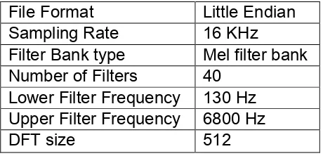
We used the executable “wave2feat” to convert the audio file from raw format to

cepstral format. The frontend parameters [35] that were considered for the

conversion are listed in table 4.1.

Table 4.1: Frontend Parameters

File Format Little Endian

Sampling Rate 16 KHz

Filter Bank type Mel filter bank

Number of Filters 40

Lower Filter Frequency 130 Hz

Upper Filter Frequency 6800 Hz

Apart from the speech inputs that were recorded using the microphone to create

the test and training databases, we also used Alphanumeric database (AN4) [33]

and Research management database (RM1) which include test and training

utterances containing files in both raw and cepstral format. We used the AN4

small vocabulary speech database containing utterances recorded at Carnegie

Mellon University circa 1991 that had candidates speak and spell out random

word sequences. We also used the medium vocabulary RM1 and large

vocabulary HUB4 acoustic and language models to perform the recognition and

compare the results. Once the test utterance is prepared in the right format the

batch files are updated in the speech input control file.

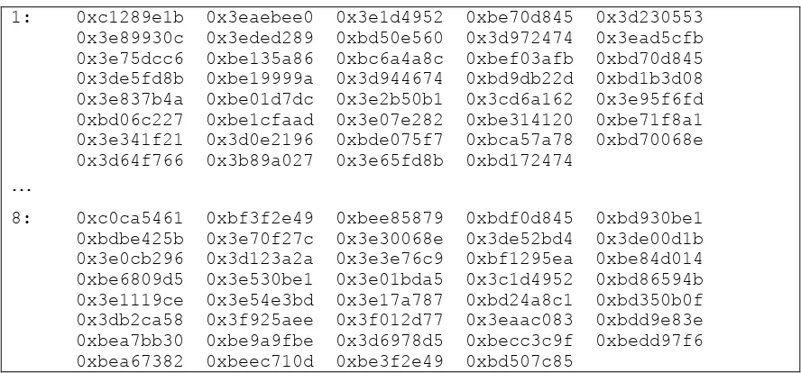
4.4 Tapping input vector files for hardware module

The test data is recognized in software using the SPHINX decoder source code.

We used a Linux platform to implement the software recognition with the input

parameter files from the acoustic models and the test data being fed from the

command line. The recognized result is compared with the actual test input data

to verify correctness and the procedure is repeated for different test input files.

We used the CSCOPE, a UNIX/Linux based tool to browse the SPHINX decoder

source code. All the procedures involved in the recognition were evaluated and

the routines which implemented the function of the hardware module described in

figure 3.2 were identified. The source code was recompiled to tap the input

vector files that are required for the hardware module. The data tapped were

then converted to 32-bit floating point data compatible to the hardware module

discussed in [2]. Tables 4.2, 4.3, 4.4 and 4.5 give all the model parameter files in