An Adaptive Cluster based routing in WSN using Energy-Position dissemination and Integer linear programming

(1)

Vol. 3, Issue 10, October 2015

Copyright to IJIRCCE DOI: 10.15680/IJIRCCE.2015. 0310175 9960

An Adaptive Cluster based routing in WSN

using Energy-Position dissemination and

Integer linear programming

Anubha Deshmukh, Ankita Gupta

M.Tech Student, Dept. of CSE, Maxim Institute of Technology, Bhopal, Madhya Pradesh, India

Assistant Professor, Dept. of CSE, Maxim Institute of Technology, Bhopal, Madhya Pradesh, India

ABSTRACT:A wireless sensor network comprises of a proportion of low-cost sensors that have an inadequate energy resource. Voluminous applications together with environment monitoring use a clustering methodology for competent energy consumption. An efficient power saving arrangement & intelligent mechanism requirements to be designed developed for the reasonable energy consumption in the WSN to improve lifetime of network. The cluster-based technique is one of significant approaches to reduce energy consumption in the WSNs. This research work is taking traditional probabilistic clustering protocol concepts; also consider heterogeneity in wireless sensor network as an effective way to increase the network lifetime and stability. We are proposing a Distributed Energy- position based clustering scheme which is also optimized through Integer Linear Programming for efficient routing in wireless sensor network, the main intention is to make an optimized cluster head selection process and adaptive cluster formation which depends upon current network conditions and resource status.To perform ideal distribution for the sensor node clusters, average distance between sensor nodes is calculated & used to select residual energy & concept of the network density for selecting appropriate clustering by the location head nodes. The lifetime of the WSN is extended by using uniform cluster location & balancing network loading among clusters. Experimental results shows that with this network designing the network lifetime and stability period increases extensively.

KEYWORDS: Wireless sensor network, Energy efficient clustering, integer linear programming, routing, Energy

Distribution, network density, Network Lifetime, Adaptive clustering.

I. INTRODUCTION

There is a wide attention towards reducing the power consumption on the Wireless Sensor Networks (WSNs). Wireless Sensor Networks (WSN)typicallycomprises of lowcostnodes having sensors, limited computation facilities, apower module and transmission segment that is accomplished ofshort radio range communication.The only source of energy isthe battery, which is unlikely to be substituted. Hence, energypreservation becomes one of the most imperative encounters in WSNs. WSN nodes are densely deployed and hence no availabilityof a scarce of them does not hinder applicationperformance. It should be revealed here that, in someapplications, for occurrence, in military applications orapplications in medical science such networks are required to be highly unswerving [1].

(2)

Copyright to IJIRCCE DOI: 10.15680/IJIRCCE.2015. 0310175 9961 Earlier research has shown that because of characteristics of wireless channels, the multihop forwarding between a data source & the data sink is frequently more energy efficient than the direct transmission. Based on power model of the specific sensor node platform, there exists the optimal transmission range that minimizes complete power consumption in network. When using such fixed transmission range in the general ad hoc networks, the energy consumption is fairly balanced, especially in the mobile networks, since data sources & sinks are characteristically supposed to be circulated throughout area where network is deployed. Though, in the sensor networks, where numerous applications require many-to-one (i.e. convergecast) traffic pattern in network, the energy imbalance becomes a very significant problem, as a hot spot is formed around data sink, or the BS. The nodes in this hot spot are essential to forward the disproportionately high amount of traffic & typically die at very early stage [4-5].

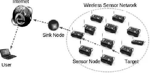
Fig. 1. Basic architecture of wireless sensor network

One of the well-known mechanisms for improving energyconservation thereby increasing the lifetime in WSN is the useof Clustering technique. Nodes of WSN are divided into anumber of groups or clusters. The coordinator of a cluster isknown as cluster-head (CH).A number of Clusteringalgorithms are discussed in literature.CHs are assumed to benodes with comparatively higher energy and so they are usedfor forwarding (may be after some computation) the datasensed by other low-energy non-CH or member nodes.

One of the key challenges of Wireless Sensor Networks (WSN) is the efficient use of limited energy resources in battery functioned sensor nodes. Hierarchical clustering [2-6] has been shown to be a promising solution to conserve sensor energy levels [7-8], above and beyond being an operative solution to organizational errands. With Cluster Heads (CH) that act as local controllers of network maneuvers, a clustered WSN has an easily manageable structure.When network is partitioned into the clusters, the data transmission can be classified into the intra- & intercluster communication i.e. thw cluster member nodes 1st send their data to cluster head, & the cluster heads send data to base station. Although the direct transmission is usually adopted for the intra-cluster communication, the multi-hop communication is more energy efficient & applicable than the single-hop communication for the inter-cluster communication [18]. Thus it is enhanced to let the cluster heads cooperate with each other to forward their data to base station.

II. WSN(WIRELESS SENSOR NETWORK)ARCHITECTURE

(3)

Copyright to IJIRCCE DOI: 10.15680/IJIRCCE.2015. 0310175 9962 base station may require accurate location of the node which is done by location finding system. The size of a single sensor node can vary from shoebox-sized nodes down to devices the size of grain of dust. [6]

Fig. 2. Basic Architecture of Wireless Sensor Network. (Ref [6])

The sensor nodes can be imagined as small the computers, extremely basic in the terms of their interfaces & their components. They typically consist of processing unit with limited the computational power & limited memory, sensors/ the MEMS (i.e. including the specific conditioning circuitry), the communication device (i.e. usually the radio transceivers/ alternatively optical), & thepower source usually in form of a battery. Other possible inclusions are the energy harvesting modules, secondary the ASICs, & possibly the secondary communication devices (for e.g. RS-232/ USB).

The base stations are 1 or more components of WSN with much more computational, energy & the communication resources. They act asgateway between sensor nodes & end user as they typically forward the data from WSN on to the server. Other the special components in routing the based networks are routers, designed to compute, calculate & distribute routing tables.

A. Classification of Sensor Network

Sensor Networks can be classified on the basis of their mode of functioning and the type of target application into two major types. They are:

a. Proactive Networks

The nodes in this network switch on their sensors and transmitters periodically, sense the data and transmit the sensed data. They provide a snapshot of the environment and its sensed data at regular intervals. They are suitable for applications that require periodic data monitoring like moisture content of a land in agriculture.

b. Reactive Networks

The nodes in this network react immediately to sudden and drastic changes in the value of the sensed attribute. They are therefore suited for time critical applications like military surveillance or temperature sensing.

B. Requirements and Design factors in Wireless Sensor Network:

Following are some of the basic requirements and design factors of wireless sensor network which serve as guidelines for development of protocols and algorithms for WSN communication architecture.

 Fault Tolerance, Adaptability and Reliability

 Power Consumption and Power management

 Network Efficiency and Data Aggregation

 Intelligent Routing

(4)

Copyright to IJIRCCE DOI: 10.15680/IJIRCCE.2015. 0310175 9963 III. REVIEW OF RELATED WORK

A number of clustering algorithms have been proposed which can be found in the survey papers [5-7]. LEACH (Low Energy Adaptive Clustering Hierarchy) [8] is a popular clustering protocol in which CHs are randomly selected. The main demerits of this scheme is that due to random selection a node with low energy may be selected as a CH and as a results its energy may get depleted very soon. Moreover, the distant nodes with little energy probably are chosen as the CHs and sometimes CHs are too close to interfere with each other. HEED [9] improves network life time over the LEACH. But, the performance of the clustering in each round imposes important overhead in network. This overhead causes the noticeable energy dissipation which results in lessening network lifetime.

Similarly many clustering algorithms are proposed like TEEN [10], APTEEN [11] and CEBCRA [12]. However, these are suffering from overhead and constructing a cluster in multiple levels is actual complex task. The Power Efficient Gathering in Sensor Information Systems i.e. PEGASIS is an energy efficient protocol [13], which affords progress on LEACH. However, PEGASIS leads to significant redundant data transmission in the network. As a result more energy consumption arises in the network. EEUC [14] (Energy Efficient Uneven Clustering) algorithm is a distributed clustering algorithm, where the CHs are elected by localized the competition. However, performing of clustering in each round of EEUC imposes significant overhead. Author of this paper has recently proposed a GA based load balanced clustering algorithm in [15] which forms clusters in such a way that the maximum load of each gateway is minimized.

They have also reported an approximation scheme for load-balanced clustering for WSNs [16]. However, being metaheuristic and approximation schemes, these algorithms do not provide optimal solution. Energy Balancing Clustering Algorithm (EBCA) has been reported in [17] to balance the energy consumption among sensor nodes which suffers from network overhead. The algorithm called LPGCRA [18] also addresses the "hot spot" problem. In order to evade premature death, it selects the CH among the normal sensor nodes which have maximum residual energy.

However, if the CH is far away from all other sensors in the cluster then all sensors in the cluster have to consume more energy including CH. Moreover, CHs transmit aggregated local data directly to the sink node which are relatively fewer in number than the total number of sensor nodes in the network, leading to rapid battery depletion in the CHs. In [19], authors proposed an algorithm to increase the lifetime of the network by optimum selection and distribution of CHs over the target area.

Moreover, in the CH selection phase CHs are selected based on the transmission time to the BS. Thus the method selects the CHs which are near to the BS in each grid and hence the member sensor nodes of the cluster deplete their energy faster for long haul transmission to the CH. In [20], various multi-hop routing algorithms have been developed. However, energy conservation of the nodes is the main concern of these algorithms. The algorithms proposed in this article takes care the energy efficiency, load balancing and improvement of the network lifetime over LPGCRA and EBCA. Previous problem consider that, the clusters near the base station also forward the information from supplementary clusters (altogether clusters need to communicate with the BS, but long-distance wireless communication ingests more energy), and as we all know, numerous members in a cluster may bring about unnecessary energy ingesting in management and communication.Hence, based on the above concerns, DSBCA algorithm [21] considers the connectivity density and the location of the node, trying to build a more balanced clustering structure.If two clusters have the same connectivity density, the cluster much farther from the base station has larger cluster radius;if two clusters have the same distance from the base station, the cluster with the higher density has smaller cluster radius.

IV. ENERGY-POSITION DISSEMINATION AND INTEGER LINEAR PROGRAMMING BASED ROUTING

(5)

Copyright to IJIRCCE DOI: 10.15680/IJIRCCE.2015. 0310175 9964 1. Cluster Head (Superior node) selection phase

We consider the sensor network that is hierarchically clustered. Our proposed algorithm keeps such the clustering hierarchy. In our protocol, clusters are re-established in each ―round.‖ The new cluster heads are elected in each round & as a result load is well distributed & balanced among nodes of network. Furthermore each node transmits to closest cluster head so as to split communication cost to sink (i.e. which is tens of times greater than processing &the operation cost.) Only cluster head has to report to sink & may expend the large amount of energy, but this occurs periodically for each node. In this protocol there is optimal percentage popt(i.e. determined a priori) of the nodes that has to become the cluster heads in

each round assuming uniform distribution of the nodes in space. A random field created and nodes are randomly placed, every node contains a specified amount of energy. Bisection between nodes through random modelling, and path-cost calculated through distance vector estimation.

In proposed work, for making global decision, residual energy of each sensor is compared with the average network energy and due to heterogeinity, proposed work also consider initial energy for the selection criteria. The initial energy of sensors are compare with the total network energy. Our aim to maximize stability and lifetime is depend upon the maximum use of more powerful CHs within network. For this we are considering sensors closer to BS and which are in denser area. So that, they can collect more data and forward to a lesser distance.

First section is the network initialization, in this phase we have to decide network parameters, such as filed area, theno. of devices, the device parameters. The routing is based on the distance vector, means we have to make the communication between our network devices through the calculation of distance in hop-by-hop manner (i.e. Node to Node communication is based on the distance vector &the node to cluster head communication is also based on the distance vector) For this, 1st of all we have to calculate the distance vector between the network devices based on their position, & path & the cost is calculate according to these the distance vectors values. Calculate probability of selection of Cluster Head sensor 𝛽from all 𝛼sensors after the trigger (random) head selection process is

𝑷𝒐𝒑𝒕 =𝐏𝐈𝐋𝐏(𝛃) ∗ 𝛂 ∗ 𝚬𝐢𝐧𝐭𝐢𝐚𝐥(𝛃) 𝚬_{𝐭𝐨𝐭𝐚𝐥}(𝛂)∗

𝚬𝑐𝑢𝑟𝑟𝑒𝑛𝑡 (𝛃) 𝚬_average (𝛂) ∗

𝛒(𝛃)

𝛔(𝛃) (1)

Total network energy is calculated by summing energies of all sensors and average energy is calculated by the

following equation: 𝚬average = 𝚬total × (

1−r 𝑐𝑢𝑟𝑟𝑒𝑛𝑡 R max

n )

Here, PILP is calculate through the integer linear programming, based upon the optimum solution of our algorithm, Eint

initially supplied energy with respect to total energy Etot and Ecurr is current resource status with respect to average energy

in network𝚬average . 𝛒(𝛃) And𝛔 𝛃 are the network density and distance from base station of ithsensor. We also consider

that the selection of head is also depends upon the number of sensorsn in the network as number of clusters is directly proportional to the number of sensors in network.The best sensor node select within the network

whose𝚬𝐢𝐧𝐭𝐢𝐚𝐥(𝛃)

𝚬_{𝐭𝐨𝐭𝐚𝐥}(𝛂), 𝛒(𝛃) 𝛔(𝛃)and

𝚬𝑐𝑢𝑟𝑟𝑒𝑛𝑡 (𝛃)

𝚬average (𝛂) ratio is high, also its selection probability is also high which is decided throughPILP this is

called as network dependent conditional probability.

If random number is less than threshold T s𝑜𝑝𝑡 then the node becomes the cluster head in current round. The

threshold is set as: Where, r is current round no. (i.e.,starting from round 0.) The election probability of the nodes Є G to become the cluster heads increases in each round in same epoch & becomes equal to 1 in last round of epoch. Note that by the round we define the time interval where all the cluster members have to transmit tothe cluster head once. We show in this paper how election process of the cluster heads should be adapted appropriately to deal with theheterogeneous nodes, which means that not all nodes in field have the similar initial energy. Let, 𝜏𝑡𝑒𝑚𝑝is a temporary random number(0 to 1)

allotted to every node 𝜏𝑡𝑒𝑚𝑝 ≤ T s𝑜𝑝𝑡 . The sensor 𝛽 should select as head.

Where, T s𝑜𝑝𝑡 =

P𝑜𝑝𝑡

1−P𝑜𝑝𝑡 rmod_{P 𝑜𝑝𝑡}1

if ∈ G

0 otherwise

(6)

Copyright to IJIRCCE DOI: 10.15680/IJIRCCE.2015. 0310175 9965 2. Automatic Cluster building phase

After selection of the cluster head, the cluster region created around particular cluster head, & the nodes belong to that region is labelled as the cluster members. In transmission phase, the Cluster members transmits their data to the cluster head &the cluster head transmit collected data to destination directly.

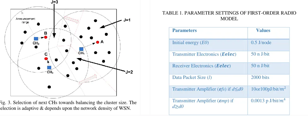
Fig. 3. Selection of next CHs towards balancing the cluster size. The selection is adaptive & depends upon the network density of WSN.

TABLE 1. PARAMETER SETTINGS OF FIRST-ORDER RADIO MODEL

Parameters Values

Initial energy (E0) 0.5 J/node

Transmitter Electronics (𝑬𝒆𝒍𝒆𝒄) 50 n J/bit

Receiver Electronics (𝑬𝒆𝒍𝒆𝒄) 50 n J/bit

Data Packet Size (l) 2000 bits

Transmitter Amplifier (𝜺fs) if d≤d0 10or100pJ/bit/𝑚2

Transmitter Amplifier (𝜺mp) if d≥d0

0.0013 p J/bit/𝑚4

This clustering is optimal in sense that the energy consumption is well distributed over all the sensors & the total energy consumption is minimum. Such the optimal clustering highly depends on energy model we use. For purpose of this study we use alike energy model & analysis as proposed in. According to radio energy dissipation the model illustrated in the Figure 4, in order to accomplish the acceptable Signal-to-Noise Ratio (SNR) in transmitting the L-bit message over the distance d, the energy expended by radio is given by:

Fig. 4. WirelessRadio Energy Dissipation Model

𝐸𝑇2 𝑙, 𝑑 =

𝐿. 𝐸𝑒𝑙𝑒𝑐 + 𝐿. ∈𝑓𝑠. 𝑑2𝑖𝑓𝑑 ≤ 𝑑𝑡𝑕𝑟𝑒𝑠 𝑕

𝐿. 𝐸𝑒𝑙𝑒𝑐 + 𝐿. ∈𝑚𝑝. 𝑑4𝑖𝑓𝑑 > 𝑑𝑡𝑕𝑟𝑒𝑠 𝑕

(3)

Here 𝐸𝑒𝑙𝑒𝑐 is energy dissipated per bit to run transmitter/ the receiver circuit, ∈𝑓𝑠&∈𝑚𝑝 depend on transmitter amplifier

model we use, &d is the distance between sender & receiver. By equating the 2 expressions at 𝑑 = 𝑑𝑡𝑕𝑟𝑒𝑠 𝑕, we

have𝑑𝑡𝑕𝑟𝑒𝑠 𝑕 = ∈𝑓𝑠/∈𝑚𝑝. To receive the L-bit message radio expends𝐸𝑅𝑥 = 𝐿. 𝐸𝑒𝑙𝑒𝑐.This radio model help here to

calculate amount of the dissipated energy after every round based on the distance vector based calculation.

Clustering & the routing procedure continues till network devices alive, devices with the proper energy levels are selected as the cluster head one after another every round. After each transmission round, the device’s residual energy is calculated with radio energy model for the wireless communication network, this helps us in deciding a cluster head node to continue transmission in the next transmission round. In case of research work in wireless network, system efficiency can be calculated from the relation of input and output data packets. Hence the throughput, end to end delay, packet delivery fraction ratio, and network lifetime are the best suited parameters to show research efficiency.

𝐸𝑇𝑋(𝐿, 𝑑 )

Transmit

Electronics

𝐸𝑅𝑋(𝐿, 𝑑 ) TX

Amplifier

Receive

(7)

Copyright to IJIRCCE DOI: 10.15680/IJIRCCE.2015. 0310175 9966 3. Integer Linear Programming

In proposed work the optimum value of user defined selection probability is calculated through ILP. The foundation of much of the analytical decision making is the linear programming. In linear program, there are variables, constraints, & an objective function. The variables,the decisions, take on the numerical values. Constraints are used to limit values to the feasible region. These constrictions must be linear in verdict variables. Objective function then defines which the particular assignment of the feasible values tovariables is optimal: it is one that maximizes (i.e. /the minimizes, depending on the kind of the objective) objective function. Objective function must also be linear in variables.The linear programs can model many problems of the practical interest, & the modem linear programming optimization codes can find the optimal solutions to problems with numerous constraints & variables. It is this combination of the modelling strength & solvability that makes the linear programming so important.

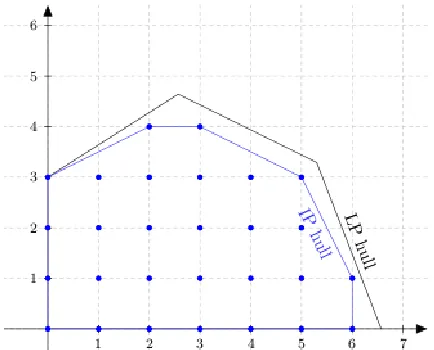
The integer programming adds additional constraints to the linear programming. An integer program begins with the linear program, & adds the requirement that some/all of variables takings on an integer value. This ostensibly innocuous change momentously increases no. of the problems that can be modelled, but also makes the models more difficult to solve. In fact, one frustrating aspect of integer programming is that two seemingly similar formulations for the same problem can lead to radically different computational experience: one formulation may quickly lead to optimal solutions, while the other may take an excessively long time to solve.A linear program (LP) is an optimization problem of the form

𝑚𝑖𝑛_𝑥∈𝑅𝑑𝑐𝑇x (4)

Subject toAx ≤ b

Fig. 5.The polygon bounded in black (including portions of the two axes) is the feasible region of the linear program relaxation (also known as the linear hull or LP hull). This is what you get if you relax the integrality restrictions while enforcing all functional constraints and variable bounds. The blue dots are the integer lattice points inside the polygon, i.e., the feasible solutions that meet the integrality restrictions. The blue polygon, the integer hull or IP hull, is the smallest convex set containing all integer-feasible solutions. The IP hull is always a subset of the LP hull. Assuming a linear objective function, one of the vertices of the IP hull (all of which are lattice points) will be the optimal solution to the problem.

If the problem is feasible, the optimum is attained at a vertex of the polyhedron that defines the constraint space. If we add the constraint x ∈𝕫𝑑_{, then the above is called an}_{integer linear program}_{(ILP). For some special parameter settings—e.g.,}

when b is an integer vector and A is totally 𝑢𝑛𝑖𝑚𝑜𝑑𝑢𝑙𝑎𝑟—all vertices of the constraining polyhedron are integer points; in

(8)

Copyright to IJIRCCE DOI: 10.15680/IJIRCCE.2015. 0310175 9967 V. RESULTS

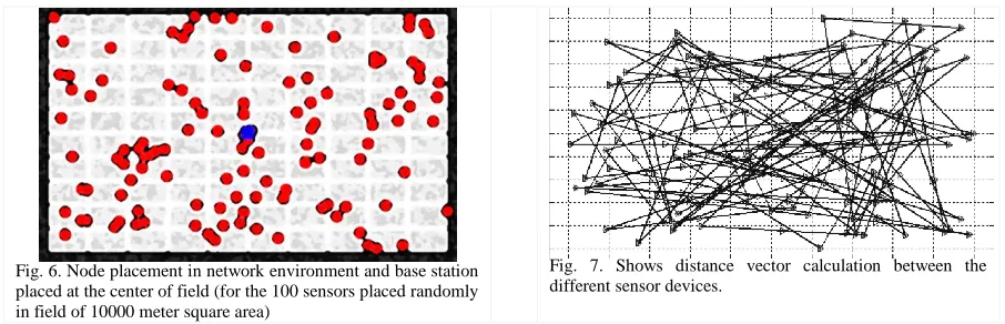
This work is apply Method in a Sensor Field of Area 100×100 m. However one can change the field area as per the result variations. Also, base Station is Placed at Centre of Sensor Field initially, however we can change the Position of base Station. Initially dissipated energy is Zero and the residual energy is Amount of the initial energy in a Node, Therefore the Total energy 𝐸𝑡 also Amount of the residual energy because it is sum of the dissipated and the residual energy. Simulations

are carried out in theMATLAB R2015a.

Fig. 6. Node placement in network environment and base station placed at the center of field (for the 100 sensors placed randomly in field of 10000 meter square area)

Fig. 7. Shows distance vector calculation between the different sensor devices.

After starting a round, firstly it checks if there is a dead node in the Sensor Field, and repeats these criteria after every round. Election of Cluster Heads for member nodes and a cluster head node are done in different loops which depend on the Election Probability used. After a Cluster Head sent its Data to Sink, Energy dissipated is calculated, through energy models considered in the propose work, in order to calculate how much energy dissipated after a steady state and whether a Cluster head is eligible to transmit data in the next round too. This Energy thoroughly depends upon the distance between BS and CH for CH, and Member node to CH for Member node. The 100 Nodes are placed in randomly manner in whole field, the no. of the clusters directly depends upon number of the cluster head. A single CH is consigned to the clusters which act as sub-destination &the route data from further cluster member nodes to destination (i.e. Sink or Base Station).

The distance vector calculation is very significant process while developing the communication protocol for the sensor network, as energy is unswervingly reliant on to distance, so it is necessary for system to calculate distance between all the sensor devices with each other. Let assume that node position in cell is (xn, yn). It can be defined distance between

node i & the other node (xc, yc) as:D[i]= (xc− xn)2+ (yc− yn)2

Throughput of receiving bits:It is ratio of the total no. of the successful packets in bits received at sink or the BS in a specified aggregate of time. And, End-to-End Delay: It is adjournment that could be instigated by buffering during the route discovery, queuing delays at the interface queues, the retransmission delays at the media, &propagation & transfer times.D𝑒𝑒=_{Total Number of Data Packets Recieved}Current Transmission period .

In Proposed model, the Node will becomes Cluster Head, if Temporary number (between 0 - 1) assigned to it is less than Probability Structure Below,

𝑇 𝑠𝑖 =

𝑃𝑖

1 − 𝑃𝑖 𝑟𝑚𝑜𝑑 1 𝑃𝑖

𝑖𝑓 ∈ 𝐺

0 𝑜𝑡𝑕𝑒𝑟𝑤𝑖𝑠𝑒

(9)

Copyright to IJIRCCE DOI: 10.15680/IJIRCCE.2015. 0310175 9968 Fig. 8. The graph above shows the comparative view of obtained network

throughput from both proposed scheme & the LEACH &the Protocol proposed by Ying Liao [21]. Throughput obtained with respect to no. of the rounds or communication period. It is measured in the terms of bits/second. Above experiment are done for the 100 sensor nodes in field area.

Fig. 9. The graph obtained shows comparison of end to end delay measured at base station/ the delay introduced by routing scheme in delivering the data packets to the base station from both proposed scheme & the LEACH & the Protocol proposed by Ying Liao [21]

After the higher weight node becomes the Head, Wireless radio Energy Model are used to estimate Aggregate of Energy Disbursed by it on that Particular Round & complete the round of steady state phase. When the node residual energy is zero then node is called dead & is terminated from network environment.

Fig. 10. Figure above shows the comparative view of death of the sensor nodes with each round for both proposed scheme & the LEACH &the Protocol proposed by Ying Liao [21] for 100 sensor nodes in the field area.

Fig. 11.Figure above shows a comparative view of death of sensor nodes with each round for both proposed scheme & LEACH and Protocol proposed by Ying Liao [21] schemes for 25 sensor nodes in the field area.

Result is taken when the base station is placed at the center of sensor field and the selection probability is defined through the energy values considered. It is clear from the figure that both the network lifetime and stability of lifetime of network is achieved through proposed protocol. Also, it was observed that the technique network proposed in LEACH and Protocol proposed by Ying Liao [21] completely stopped functioning at an earlier simulation rounds compared to our proposed technique. We saw that the functional capacity for LEACH and Protocol proposed by Ying Liao [21] created network lasted till an estimated value of +1300 rounds of simulation, while the functional capacity of the proposed approach lasted till an

0 500 1000 1500 2000 2500 3000 3500 4000 4500 5000 0 2 4 6 8 10 12 14x 10

4

x(Number of Rounds)

y (Th ro u g h p u t (b it s )) LEACH protocol Protocol By Ying Liao Proposed Protocol

0 500 1000 1500 2000 2500 3000 3500 4000 4500 5000 0 0.05 0.1 0.15 0.2 0.25 0.3 0.35 0.4 0.45

x(Number of Rounds)

y (E n d t o E n d D e la y ) LEACH protocol Protocol By Ying Liao Proposed Protocol

0 500 1000 1500 2000 2500 3000 3500 4000 4500 5000 0 10 20 30 40 50 60 70 80 90 100

x(Number of Rounds)

y (L if e ti m e o f S e n s o r N e tw o rk ) LEACH protocol Protocol By Ying Liao Proposed Protocol

0 500 1000 1500 2000 2500 3000 3500 4000 4500 5000 0 5 10 15 20 25

x(Number of Rounds)

(10)

Copyright to IJIRCCE DOI: 10.15680/IJIRCCE.2015. 0310175 9969 estimated value of +3000 rounds of simulation. Statistics of the dead nodes with respect to transmission the rounds is shown in figure below:

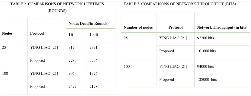
TABLE 2. COMPARISONS OF NETWORK LIFETIMES

(ROUNDS)

Nodes Protocol

Nodes Dead(in Rounds)

1% 100%

25 YING LIAO [21] 312 2391

Proposed 2285 3756

100 YING LIAO [21] 906 1376

Proposed 2497 2128

TABLE 3. COMPARISONS OF NETWORK THROUGHPUT (BITS)

Number of nodes Protocol Network Throughput (in bits)

25 YING LIAO [21] 92200 bits

Proposed 101000 bits

100 YING LIAO [21] 94000 bits

Proposed 128000 bits

This section conclude that and also here results shows that, this protocol successfully extends stable region to more than 2000 rounds by being aware of the heterogeneity through assigning probabilities of the cluster-head election weighted by relative initial energy & the geographical position of the nodes, also lifetime of the network protracted to over and above 3000 rounds in this protocol.

VI. CONCLUSION

This proposed work was carried out with extensive evaluations in the cooperative multi-path routing problem to save power consumption while satisfying the bandwidth requirement. Many problems are considered from previous work including, the self-organizing concept, weight for selection of head etc. This work proposed ―An Adaptive Cluster based routing in WSN using Energy-Position dissemination and integer linear programming‖, which is further compared by the Load-Balanced Clustering Algorithm withthe Distributed Self-Organization for the Wireless Sensor Networks proposed by 𝑦𝑖𝑛𝑔 𝑙𝑖𝑎𝑜 in [21]. This protocol is used to determine optimal probability for the cluster formation in the WSNs. As simulation results show that in the terms of network lifetime of the sensor node, since the use of optimal probability yields the optimal energy-efficient clustering.

(11)

REFERENCES

1. 𝑃𝑒𝑟𝑖𝑙𝑙𝑜, Z. Cheng, and W. Heinzelman, ―On the problem of unbalanced load distribution in wireless sensor networks,‖ in Proceedings of the Global

Telecommunications Conference (GLOBECOM) Workshop on Wireless Ad Hoc and Sensor Networks, 2004.

2. A. A. Abbasi and M. Younis, ―A survey on clustering algorithms for wireless sensor networks,‖ Computer Commun., vol. 30, pp. 2826–2841, 2007. 3. S. Bandyopadhyay and E. J. Coyle, ―An energy efficient hierarchical clustering algorithm for wireless sensor networks,‖ in Proc. INFOCOM, Mar.

2003.\

4. I. Matta, G. Smaragdakis, and A. Bestavros, ―SEP: a stable election protocol for clustered heterogeneous wireless sensor networks,‖ in SANPA, Aug. 2004.

5. L. Qing, Q. Zhu, and M. Wang, ―Design of a distributed energy-efficient clustering algorithm for heterogeneous wireless sensor networks,‖ Computer Commun., vol. 29, pp. 2230–2237, 2006.

6. A. A. Abbasi, M. Younis, ―A survey on clustering algorithms for wireless sensor networks,‖ Computer Commun., Vol. 30, pp. 2826-2841, 2007. 7. Xuxun Liu, ―A Survey on Clustering Routing Protocols in Wireless Sensor Networks,‖ Sensors, Vol. 12, pp. 11113-11153, 2012.

8. W. Heinzelman et al., "Energy-Efficient Communication Protocol for Wireless Mircrosensor Networks," Proc. of Int. Conf. HICSS 2000, pp. 3005-3014, 2000.

9. Younis, O. Fahmy, S. ―HEED: A hybrid, energy-efficient, distributed clustering approach for ad-hoc sensor networks,‖ IEEE Trans. Mobile Comput, Vol. 3, 216–379, 2004.

10. Manjeshwa et al., ―TEEN: A Routing Protocol for Enhanced Efficiency in Wireless Sensor Networks,‖ In Proc. IPDPS 2001, pp. 2009–2015, 2001. 11. Manjeshwar, E. Agrawal, D. P., ―APTEEN: A Hybrid Protocol for Efficient Routing and Comprehensive Information Retrieval in Wireless Sensor

Networks,‖ In: Proc. of IPDPS 2002, pp. 195–202, 2002.

12. Pratyay K, Prasanta KJ, ―An energy balanced distributed clustering and routing algorithm for wireless sensor networks,‖ Proc. of Int. conf. PDGC 2012, IEEE Xplore, pp 220–225, 2012.

13. S. Lindsey, C.S Raghavendra, ―PEGASIS: Power efficient gathering in sensor information systems‖, Proc. IEEE Aerospace and Electronic Systems Society, pp. 1125-1130, 2002.

14. Li C.F. et al., ―An Energy-Efficient Unequal Clustering Mechanism for Wireless Sensor networks,‖ Proc. Int. Conf. MASS, pp. 596–604, 2005. 15. Pratyay K, Suneet KG, Prasanta KJ, ―A novel evolutionary approach for load balanced clustering problem for wireless sensor networks,‖ Swarm and

Evolutionary Computation, Vol. 12 pp. 48-56, 2013.

16. Pratyay K. et al., ―Energy efficient load-balanced clustering algorithm for wireless sensor networks,‖ Procedia Technology, 6, pp. 771–777, 2012. 17. L. L et al., ―Energy Balancing Clustering Algorithm for Wireless Sensor Network,‖ In: proc: NSWCTC 2009, pp. 61-64, 2009.

18. W. Liu et al., ―A Low Power Grid-based Cluster Routing Algorithm of Wireless Sensor Networks,‖ IEEE IFITA, Vol. 1, pp. 227-229, 2010. 19. Aswatha Kumar M. et al., ―Energy Efficient Clustering and Grid Based Routing in Wireless Sensor Networks,‖ Proc: of ICAdC, AISC 174, pp. 69–

74, 2013.

20. Jin, Y et al., ―Eeccr: An energy-efficient m-coverage and n-connectivity routing algorithm under border effects in heterogeneous sensor networks‖, IEEE Transactions on Vehicular Technology, Vol. 58, no. 3, pp. 1429–1442, 2009.

21. Ying Liao, Load-Balanced Clustering Algorithm with Distributed Self-Organization for Wireless Sensor Networks, IEEE SENSORS JOURNAL, , MAY 2013.

BIOGRAPHY

Anubha Deshmukh is a Research Assistant in the Computer Science & Engineering Department, College of Maxim Institute of

Technology, RGPV University. She received Master of Technology (M.TECH) degree in 2015 from RGPV, BHOPAL, India. Her research interests are Computer Networks (wireless Sensor Network) Networks), Algorithms, MATLAB R2013b (version 8.2.0.703).

Ankita Gupta is an Assistant Professor in the Computer Science & Engineering Department, College of Maxim Institute of Technology,