ABSTRACT
TABRIZIAN, PAYAM. Integrating Geospatial Computation, Virtual Reality and Tangible Interaction to Improve Landscape Design and Research. (Under the direction of Dr. Perver Baran and Dr. Ross
Meentemeyer).
Geospatial computation, visualization and user interaction technologies can transform the practice and research of environmental design to cope with the new environmental and societal problems at hand, weaving across disciplines, bridging the science and aesthetics, while introducing efficiency, flexibility, legibility and interconnectivity. In this dissertation, I leverage these technologies to develop
methodologies for enhancing research and design of environments. These methodologies aim to facilitate more efficient and accurate analysis of landscape spatial and experiential (e.g., aesthetic, restorative qualities) characteristics, and enable intuitive interaction and immersive visualization of design phenomena across spatial and temporal scales. The first methodology combines automated viewscape modeling–geospatial analysis of visible structure and patterns– with human subjective evaluations to quantify, model, and map landscape characteristics and experience of landscapes. For more accurate and granular analysis of landscape structure and pattern, I utilize high-resolution surface models derived from lidar data, and enhanced vegetation modeling is applied. To better represent in-situ conditions and capture human perceptions, I utilize photorealistic Immersive Virtual Environments (IVE), also called Virtual Reality (VR) or Immersive VR (IVE). I apply this method to model and map visual characteristics and restorative qualities of an urban park. The second methodology focuses on real-time coupling of 3D modeling and rendering, geospatial analysis, and tangible interaction allowing users to design
environments using their hands, and in real-time, receive maps and numeric feedbacks of spatial analysis, and see 3D visualizations rendered on a display or immersive head mounted displays. With this
technology designers, experts and public can collaboratively explore design alternatives through an iterative process of ideation, geocomputational analysis, realistic rendering, critical analysis, and aesthetic exploration. The methodologies and software created as part of this dissertation can be used not only in environmental design and research but also for teaching and game development. While the presented case-studies are focused on site scale urban environments, solutions can be transferred to other contexts and scales.
Integrating Geospatial Computation, Virtual Reality and Tangible Interaction to Improve Landscape Design and Research
by Payam Tabrizian
A dissertation submitted to the Graduate Faculty of North Carolina State University
in partial fulfillment of the requirements for the degree of
Doctor of Philosophy
Co-majors: Geospatial Analytics
Design
Raleigh, North Carolina 2018
APPROVED BY:
_______________________________ _______________________________
Perver K. Baran Ross K. Meentemeyer
Co-Chair of Advisory Committee Co-Chair of Advisory Committee
_______________________________ _______________________________
Helena Mitasova Christopher Mayhorn
_______________________________ _______________________________
Andrew Fox Deni Ruggeri
DEDICATION
BIOGRAPHY
AKNOWLEDGMENTS
First and foremost, I would like to thank my co-advisors, Perver Baran and Ross Meentemeyer, for all their great help and support and for being always ready to discuss new ideas. My appreciation equally goes to Helena Mitasova for her valuable input and directions and more importantly, for giving me the great
TABLE OF CONTENTS
LIST OF TABLES ... viii
LIST OF FIGURES ... ix
Chapter 1: Introduction ... 1
References ... 4
Chapter 2:Modeling visual characteristic of urban landscape with viewscape analysis of lidar surfaces and immersive virtual environments ... 6
Introduction ... 7
Methods ... 10
Study area ... 10
Viewscape modeling ... 11
Immersive Virtual Environment (IVE) Survey... 16
Viewscape model assessment ... 19
Results ... 19
Discussion ... 20
Predicting visual characteristics ... 22
Methodological contributions and consideration ... 24
Limitations and future work ... 25
Conclusion ... 27
References ... 28
Chapter 3: Modeling restorative viewscapes: spatial mapping of urban Landscape’s restorative potential using viewscape modeling and photorealistic immersive virtual environments ... 32
Introduction ... 33
Methodology ... 35
Study area ... 35
Viewscape analysis ... 36
Computing viewscape metrics ... 39
Restoration potential survey ... 41
Stimuli... 41
Survey instrument ... 41
Procedure ... 42
Data analysis ... 43
Mapping restorative potential ... 43
Results ... 44
Restoration potential survey ... 44
Restorative potential map ... 45
Discussion ... 48
Methodological considerations ... 48
Perceived restoration potential model ... 51
References ... 54
Chapter 4: Tangible Immersion for Ecological Design ... 58
Abstract ... 59
Introduction ... 60
Background ... 60
Tangibles... 60
Immersion ... 60
Methods ... 61
Tangible Landscape ... 61
3D Planting and Realistic Rendering ... 62
Case study ... 63
Results and reflections ... 64
Conclusions ... 67
References ... 67
Chapter 5: Real-time 3D Rendering and Immersion with Tangibles Landscape ... 69
.Blender ... 70
Hardware and Software Requirements ... 71
Software Architecture ... 72
File Monitoring ... 73
3D Modeling and Rendering ... 73
Handling Geospatial Data ... 74
Object Handling and Modifiers ... 75
3D Rendering ... 77
Materials ... 79
Workflows ... 81
Realism and Immersion ... 84
Realism ... 84
Virtual Reality Output ... 85
Tangible Landscape Add-on in Blender ... 86
References ... 87
Integrating Tangible and 3D Modeling Methods ... 88
Case Study: Designing a Park ... 92
Site Description and Model ... 92
Scenario 1 ... 92
Scenario 2 ... 95
Evaluation of Scenarios ... 95
References ... 98
Chapter 6: Conclusion ... 99
Urban viewscapes ... 100
Potentials and opportunities for planning and design ... 100
Software availability and replicability ... 103
Realtime 3D visualization and immersion with Tangible Landscape ... 104
Implications for Design ... 104
Transferability across applications and scales ... 104
Improving the design process ... 106
Implications for teaching ... 108
Accessibility, usability and reliability ... 109
User studies ... 111
References ... 113
APPENDICES ... 115
Appendix A. Land cover map ... 116
Appendix B. Landscape metrics ... 117
Appendix C. Descriptive statistics of viewscape metrics computed for selected viewpoints... 118
LIST OF TABLES
Table 2.1 Multiple linear regression models for the three visual charactristics ... 21
Table 2.2 Descriptive statistics of visual charactristics survey ... 22
Table 3.1 Descriptive statistics of restoration potential survey ... 45
Table 3.2 Results of the multiple linear regression analysis for the RP... 46
LIST OF FIGURES
Figure 2.1 Representation of deciduous trees in lidar derived DSM ... 9
Figure 2.2 Location of the study site ... 11
Figure 2.3 Land cover fusion process ... 12
Figure 2.4 Site photography and lidar points for three dominant vegetation structures ... 13
Figure 2.5 Trunk obstruction modeling process and results ... 14
Figure 2.6 Procedure for computing viewscape metrics ... 15
Figure 2.7 Procedure for creating immersive scenes ... 16
Figure 2.8 Equirectangular images used in IVE survey. ... 17
Figure 3.1 Location of the study site ... 36
Figure 3.2 Digital surface interpolated from lidar points ... 37
Figure 3.3 Representation of viewshed map before and after trunk obstruction modeling ... 38
Figure 3.4 Process of generating the lancover through fusion of spatial data ... 39
Figure 3.5 3D representation of maps generated in the process of viewscape analysis ... 40
Figure 3.6 Panoramic photos used in the IVE survey. ... 42
Figure 3.7 Perceived restoration potential map of the Dorothea Dix park, Raleigh, NC... 47
Figure 3.8 Viewscape characteristics of Dorothea Dix park, Raleigh, NC ... 48
Figure 4.1 Collaboratively designing and immersively visualizing a park with Tangible Landscape ... 59
Figure 4.2 Tangible Landscape physical setup ... 61
Figure 4.3 Software architecture for coupling GRASS GIS and Blender. ... 62
Figure 4.4 Interaction modes supported in Tangible Landscape ... 63
Figure 4.5 Hydrological map and topographic contours projected in Tangible Landscape ... 64
Figure 4.6 Classified landcover map and biodiversity analyses projected in Tangible Landscape ... 64
Figure 4.7 Plan and profile of the boardwalk projected in Tangible Landscape ... 64
Figure 4.8 The Landscape architect's design process... 65
Figure 4.9 The geoscientist and landscape architects's design process ... 66
Figure 5.1 Tangible Landscape phsyical setup ... 71
Figure 5.2 Tangible Landscape’s software architecture ... 72
Figure 5.3 Three modes of 3D rendering in Blender ... 78
Figure 5.4 Modeling and shading procedure for coverting a raster map to 3D water feature ... 80
Figure 5.5 Assigning textures map to an imported raster surface ... 81
Figure 5.6 The process for modeling and shading a terrain feature... 82
Figure 5.7 The process for modeling and shading vegetation ... 83
Figure 5.8 The process for modeling and shading a trail feature ... 84
Figure 5.9 Viewport rendering of the Blender scene with two modes of realism ... 85
Figure 5.10 Tangible Landscape addon in Blender ... 86
Figure 5.11 Case study appartus ... 88
Figure 5.12 Study area with the highlighted physical model extent... 91
Figure 5.13 Design scenario 1: landform and hrdrology ... 92
Figure 5.14 Design scenario 1: vegetation and trail design ... 93
Figure 5.15 Design scenario 2: design process and rendering output ... 95
Figure 6.1 Process for maipulation of photorealistic IVE images... 102
Figure 6.2 Head tracking and physiological recording during immersion... 103
Figure 6.3 Examples of simulation and visual effects in Blender... 104
Figure 6.4 Rendering of the FUTURES simulation ... 106
Figure 6.5 Walkthrough animation of a trail designed with Tangible Landscape... 106
Figure 6.6 Examples of Tangible Landscape applications in teaching... 108
Figure 6.7 Examples of three rendering modes in Tangible Landscape ... 109
CHAPTER 1
Introduction
The pernicious problem that we as designers face today is that we tend to use old tricks to deal with new challenges. In other words, we tend to perpetuate structures of disciplinary knowledge that had been shaped around earlier problems but that no longer correspond to the problems at hand. The fields that constitute urban studies today—development, design, community, and environment— do not effectively reflect the complexity of today’s urban problems. Neither do those that constitute architecture —design, building technology, and culture studies. Problems such as coastal flooding, wildfire, transportation, material scarcity, mental and physical health, environmental injustice, and efficiency straddle across scales and disciplines, and demand new tools and new tricks.
An effective approach to urban landscape planning and design require seamless integration of spatial and experiential analyses (Gobster, et al., 2007; Kovacs, et al., 2006; Wang, et al., 2016a). The former is essential for quantifying, preserving, and promoting natural processes and resource values that are – directly or otherwise– related to humans’ physiological and psychological well-being. The latter is as important, if not more, as experience influences people’s engagement and use of landscape, as well as public support for any landscape change (Fry, et al., 2009; Gobster, et al., 2007; Wang, et al., 2016a). We are more likely to support and preserve landscapes in which we have positive experiences. Conversely, we tend to alter or neglect landscapes with lower perceived qualities, irrespective of their ecological significance (Fry, et al., 2009; Gobster, et al., 2007; Kullmann, 2016). So far, with some limited exceptions, the spatial and experiential dimensions have not been effectively integrated in landscape design and research (Gobster, et al., 2007; Wang, et al., 2016b). This partly stems from disparities that exist between expertise domains (e.g., ecology vs. psychology), scale (landscape-scale vs. human-scale), analysis tools (e.g., GIS vs. surveys), and representation tools (e.g., metrics, maps vs. images, 3D simulations; Kullmann, 2016).
deal with the new problems at hand, weaving across disciplines and sub-disciplines, introducing speed, flexibility, legibility and interconnectivity among the different aspects of the design domain. They can also contribute to making our fields more flexible to change and adapt to the new sets of problems as they emerge.
With geospatial computation technologies, we can precisely model urban landscape’s structure and patterns, explore the relationship between urban landscape form and its performance (e.g., biodiversity, pollution remediation, mobility, connectivity and visual impacts) across temporal and spatial scales. Flexibility of the geospatial modeling and simulation tools has empowered us to develop automated workflows for assessing not only the existing but also the emerging and proposed landscapes. Over the years, environmental design fields have incredibly advanced to consider form, composition, and program essential, to leave out technical issues and performance as contingent or unpredictable. The computational process allows us for more contingency to enter into the design process.
With state-of-the-art geovisualization technologies such as virtual reality and immersive virtual environments (IVEs), we can better understand and communicate “real world” experiences of existing landscapes or generate photorealistic “what if” scenarios for a changing landscape. These game-like environments can be flexibly programmed to implement interactions (e.g., walking) while collecting subjective (e.g., surveys) and objective (e.g., physiological sensors, and eye-tracking) response data. This allows us to rigorously assess how exposure to different landscape patterns and structures influence a range of behavioral (e.g., physical activity), perceptual (e.g., aesthetic enjoyment and safety), affective (e.g., mood and stress) and cognitive (e.g., direct attention recovery, learning, and creativity) responses. Advance user interaction technologies, such as tangible user interfaces, facilitate more engaging and intuitive exploration of spatial data and visualization, and by doing so bridge the interdisciplinary and knowledge divides allowing designers, engineers, and public to collaboratively steer and decide about design scenarios.
Integrating these emerging technologies enables researchers and designers to cross the disciplinary divides between the research of human experience and the environment. It affords researchers to
In this dissertation, I explore methodologies that integrate geospatial computation, IVEs, and tangible user interfaces with aims to (1) facilitate more efficient and accurate analysis of landscape spatial and
experiential (e.g., aesthetic, restorative qualities) characteristics, and (2) enable intuitive interaction and immersive visualization of design phenomena across spatial and temporal scales. While the proposed methodologies are applicable in other environmental design application and scales, the contextual focus of this dissertation is site-scale mixed use urban environments (i.e., urban parks). In chapters 2 and 3, I present a methodology for modeling experiential qualities of urban environments through an integrated approach that combines objective and perception-based landscape assessment approaches. I relate geospatial analysis of visible landscape structure and pattern (viewscape) with a survey of human
perceptions. To account for fine-grain urban structure, I propose a number of improvements in geospatial analysis, and human perception elicitation techniques such as using high-resolution surface models derived from lidar data, enhanced vegetation modeling, and using photorealistic IVEs to elicit
perceptions. In chapter 2, I describe the workflow and implementation of the viewscape model in GIS, and evaluate its explanatory power to predict visual characteristic (visual access, naturalness, complexity) by comparing the model results with human subjects’ rating of IVEs. In chapter 3, I apply the developed viewscape analysis method to predict and map perceived restoration potential of urban environments. I investigate the landscape structure and pattern indices that predict restoration potential and apply the relationships to generate spatially explicit maps of restoration potential.
In chapters 4 and 5, I present a methodology and software for real-time 3D rendering with geospatial analysis and tangible interaction- a first solution for generating on-the-fly realistic renderings of changing geospatial data and simulations, informed by tangible interaction, and with live output for head-mounted-displays. The proposed approach uses Tangible Landscape system (Petrasova, et al., 2018) which runs on open source geospatial analysis (GRASS GIS) software coupled with a scanner and projector. Tangible Landscape is paired with an open source 3D modeling and rendering software (Blender) to convert geospatial data and analysis to realistic 3D rendering, enabling traditional bird’s-eye views of
environments to be visualized at ground-level in virtual reality. This coupling allows landscape architects, other professionals, and the public can collaboratively explore design alternatives through an iterative process of intuitive ideation, geocomputational analysis, realistic rendering, critical analysis, and aesthetic exploration.
Chapter 4 introduces the methodology and demonstrates its functionality through an exploratory test-case. I provide a background to tangible geospatial interfaces and current state of the landscape design
interdisciplinary problem solving in which a landscape architect and a geoscientist use Tangible Landscape to collaboratively design landforms, hydrologic systems, planting, and a trail network for a brownfield site.
Chapter 5 provides a technical description of the methodology and its implementation as add-on software for Blender. I describe the software architecture, the coupling mechanism, and detailed workflow for converting various types of geospatial data to 3D models and rendering. Workflows are presented as step-by-step procedures accompanied by python scripts. The chapter concludes with a small test case wherein a designer and an engineer interact with the system to design a landscape.
References
Fry, G., Tveit, M. S., Ode, & Velarde, M. D. (2009). The ecology of visual landscapes: Exploring the conceptual common ground of visual and ecological landscape indicators. Ecological Indicators, 9(5), 933–947.
Gobster, P. H., Nassauer, J. I., Daniel, T. C., & Fry, G. (2007). The shared landscape: What does aesthetics have to do with ecology? Landscape Ecology, 22(7), 959–972.
Kovacs, Z. I., Leroy, C. J., Fischer, D. G., & Lubarsky, S. (2006). How do Aesthetics Affect our Ecology? Ecology, 10, 61–65.
Kullmann, K. (2016). Disciplinary convergence: landscape architecture and the spatial design disciplines. Journal of Landscape Architecture, 11(1), 30–41.
Petrasova, A., Harmon, B., Vaclav, P., Tabrizian, P., & Mitasova, H. (2018). Tangible Modeling with Open Source GIS (2nd ed.). New York: Springer International Publishing.
CHAPTER 2
Modeling visual characteristic of urban landscape with viewscape analysis of lidar surfaces and immersive virtual environments
Preprint
This chapter is a preprint.
Attribution
I performed literature review, carried out the geospatial analysis and survey, processed data, and prepared the manuscript. Perver Baran provided the overall guidance and reviewed the manuscript. Helena
Introduction
The visual characteristics of landscapes are increasingly linked to people’s perceptual, affective and cognitive processes (Ode, & Miller, 2011; Tveit, et al., 2006). Characteristics such as complexity, openness, coherence, and naturalness, within a view, all contribute to aesthetic appreciation, perceptions of safety, perceived psychological well-being, and even mood (Barton, et al., 2009; Hipp, et al., 2015; Jansson, et al., 2013; Roe, et al., 2013). Modeling and quantifying these visual attributes as means to identify and safeguard valued landscapes and to assess public’s reactions to landscape changes has been focus of both theoretical and applied research (Gobster, et al., 2007; Palmer, 2004). Conceptual models of landscape character (Tveit, et al., 2006) have synthesized evidence from environmental psychology and principles of landscape ecology to develop measurable indicators that describe visual characteristics in terms of configuration and composition of landscape features and patterns. For example, complexity (diversity of elements and visual richness) can be expressed by variations in surface elevation, quantity and diversity of visible landcover, and shape complexity of the visible edges. These indicators can be obtained by in situ observations and landscape photographs (Arriaza, et al., 2004; Otero Pastor, et al., 2007), or through GIS modeling (Cavailhès, et al., 2009; Sang, et al., 2008; Schirpke, et al., 2013). The former approach provides a wealth of information but is restricted to the survey sites (Palmer, &
Hoffman, 2001). On the contrary, the latter approach that uses digital spatial data allows for calculation of the visual characteristics for the entire study using automated procedures and creating spatial maps of visual characteristics and quality. However, GIS-based measurements have limited correspondence with visual landscape as viewed by the observer (Ode, et al., 2010; Sang, et al., 2008).
configuration of visible landscape (e.g., pattern diversity, shape complexity, terrain ruggedness) using landscape metrics analysis tools that are commonly used in landscape ecology. A few studies that applied this method have reported good level of prediction. For example, Schirpke et al.’s (2016) model predicted 87% of variation in aesthetic potential in mountainous areas in Central Alps while Sahraoui et al.’s (2016) model explained 90% percent of variation in French urban fringes.
While viewscape models have been increasingly used to assess landscape characteristics across continental, regional, and landscape scales, their application for modeling perceptions in urban
environments, particularly at the site scale, remains largely unexplored. In contrast to commonly studied biomes such as tundra, savannah, and flat pasture that involve long-range vistas, and homogenous landcover, urban landscapes involve variety of view ranges and spatial conditions —shaped through interaction of granular landform and heterogeneous landcover. Due to difficulties in accessibility and processing lidar data for large regions, current viewscape models often utilize low-resolution DSMs or DTMs with manually extruded vegetation patches and building footprints (Sahraoui, Clauzel, et al., 2016). This is in spite of the well documented influence of spatial data resolution on accuracy of visibility analysis.(Klouček, et al., 2015; Sang, et al., 2008; Vukomanovic, et al., 2018). For example, Klouček et al. (2015) showed that coarser DSMs tend to overestimate visibility compared to fine grained lidar DSMs, and that these errors are more pronounced in smaller viewsheds.
Similar limitations hold for landcover data that is also integral for realistic estimation of visible content (e.g., number of visible deciduous trees and residential buildings), as well as for accuracy of landscape metric analysis (reviewed in Barry & Elith, 2006, Moudrý & Šímová, 2012). Publicly available landcover data are often coarse (10-30 meters) and do not represent features smaller than their pixel size (e.g., buildings, sidewalks, single trees). Although advanced methods such as object-based classification or pattern recognition exist to generate highly detailed landcover data from satellite imagery, incorporation of such data in viewscape models has been rare. To our knowledge, the only existing attempt includes the study of Wilson et al (2008) that used a 2.4 meter NDVI (obtained from QuickBird imagery) in
combination with a 1.5 meter DSM to compute visible greenness.
concept that accounts for the probability of viewing a region as determined by the spatial density and position of tree models (Llobera, 2007), or trunk obstruction modeling that replaces the trees with an approximated trunk model (Murgoitio, et al., 2017). While improvements in resolution of spatial data and vegetation obstructions modeling have separately shown promise in enhancing the accuracy of visibility analysis, to our knowledge they have not been used together in a single study to generate a high fidelity viewscape model.
Figure 2.1. Representation of deciduous trees in lidar derived DSM (left) and bird-view imagery (right) in leaf-off season.
Evaluating whether and to what extent a viewscape model measures perceived visual characteristics, and therefore whether the metrics and/or input data used are appropriate for the modeling purpose, requires comparison of the model output with human subjects’ evaluations of landscape, either in situ or through landscape photography and 3D simulations. Because in-situ measurements are often time-consuming, labor-intensive and involve several confounding factors (e.g., changing weather), research has widely resorted to online or desktop surveys using photographs and 3D simulations (Sahraoui, Youssoufi, et al., 2016). However, the use of digital stimuli is being increasingly contested for their representation validity, that is the observer’s “response equivalence” between in situ experience of landscape and a photographic representation (Palmer, & Hoffman, 2001). The least response equivalency has been reported for
photographs of heterogeneous landscapes and mixed use urban environments (Palmer, & Hoffman, 2001). Another obstacle for verification of viewscape models is the discrepancy of view coverage between perspective photographs and visibility analysis in GIS. Perspective photographs have limited field of view (FOV, 60o for standard 35 mm wide-angle lens) while viewshed algorithms use 360o line-of-sight
Immersive virtual environments (IVEs) that immerse the observer in a virtual environment (VE) can potentially minimize the gap between modelled viewscape and in-situ experience of urban landscape. In contrast to desktop displays where FOVs are limited, immersive displays (CAVETM or head mounted
displays, HMD) provide continuous visual feedback linked to the user’s head and body orientation
allowing them to freely explore the entire viewshed area, and actively engage with the VE. Comparison of IVEs with desktop displays has shown higher sense of immersion (Kronqvist, et al., 2016) and presence, i.e., the perception of physically being present in a non-physical world (Slater, et al., 2009). Also, IVEs elicit improved spatial perceptions (e.g., distance, depth), specially for more complex scenes (Kim, et al., 2012). IVEs have been widely adopted in geospatial sciences and urban planning applications such as 3D visualization of open map data (Çöltekin, et al., 2016), real-time 3D visualization of ecological
simulations (Tabrizian, et al., 2016), geodesign (Dias, et al., 2015), and user experience and interaction with geovisualizations. However, their use for human verification of visibility simulations, particularly viewscape modeling has been limited.
In this study, we develop and assess a novel multi-method approach for modeling visual characteristic of a mixed-use urban environment, an urban park. We use high-resolution DSM and landcover data retrieved from lidar to account for fine-grained structure and heterogeneous pattern of urban environments. Using a trunk obstruction modeling technique, we improve the vegetation visibility of the DSM. Based on the improved spatial data, we compute composition and configuration of viewscapes using automated GIS procedures. We conduct a perception survey using IVE images captured from a set of locations across the study area. Finally, we compare the metrics derived from the viewscape model with human subject’s evaluations of IVEs to assess the capacity of the model to predict visual characteristics. We specifically focus on three visual characteristics, namely, visual access, complexity and naturalness that have been widely used to objectively estimate landscape visual quality and have shown strong links with human psychological responses to environments (Kuper, 2017; Ode, et al., 2009; Ode, & Miller, 2011; Tveit, et al., 2006).
Methods
Study area
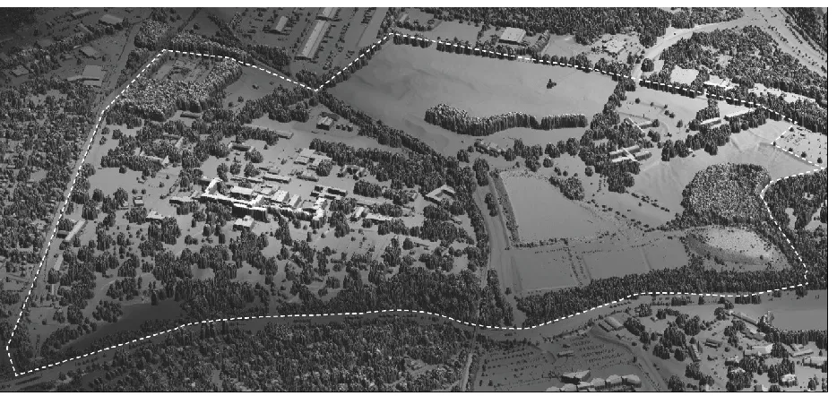
Dorothea Dix urban park covers 306 acres (125 ha) of western side of Raleigh, North Carolina (35‘46° N, 78‘39° W; Fig. 2.2). The landscape is characterized by undulating topography and heterogeneous
landcover. Vegetation coverage varies from grassy meadows, herbaceous perennials, Eastern and
numerous buildings (e.g., closed hospital, administrative and maintenance buildings, as well as derelict employee housing), and a network of paved roads. The study area therefore combines varied landscape types and spatial characteristics that makes it very relevant for our study.
Figure 2.2. Location of the study site.
Viewscape modeling
Digital surface model (DSM) and Landcover
To develop DSM and landcover we used three geospatial datasets including airborne lidar, multi spectral orthoimagery of vegetation and a road and building. The multiple return lidar data were acquired on Jan 11, 2015 (leaf-off) with average density of 2 points per m2 and fundamental vertical accuracy (FVA) of
18.2 cm. Two sets of orthoimagery were used: a 30 cm resolution orthoimagery captured in early 2015 in leaf-off condition, and a 1 m resolution four-band imagery captured in summer 2014 in leaf-on condition. DSM was developed by interpolating first-return lidar points at half-meter resolution. We used a
regularized spline with tension algorithm implemented in GRASS GIS (Mitášová & Hofierka, 1993) to balance the smoothness and approximation accuracy of the surface. The land cover was developed through fusion of three layers (Fig. 2.3):
imagery (NAIP), lidar vegetation maximum values, and Orthoimagey to classify the CHM into mixed forest, evergreen and deciduous land covers.
(2) The ground cover consisted of grasslands, herbaceous, and unpaved surfaces, which were manually, digitized these features over the 30 cm resolution orthoimagery.
(3) Buildings and paved surfaces (e.g., streets, parking surface), which were rasterized from the vector line and polygon data.
The resulting land cover map had a 0.5 m resolution (Appendix A) and included 12 land cover classes categorized based on NLCD classification.
Figure 2.3. Land cover fusion layers (a) canopy trees derived from lidar points, (b) ground cover digitized over high resolution imagery and (c) roads and buildings rasterized from official vector data are combined to generate the (d) half meter resolution land cover.
Trunk obstruction modeling
To delineate vegetation structures that required improved representation for visibility analysis, we visually inspected lidar points and field images and identified three main structures (Fig. 2.4): (1) Dense evergreen patches (mainly loblolly pines) with dense understory (mainly woody shrubs and vines), (2) Evergreen over-story mixed with deciduous midstory (mainly red maple and sweetgum), and understory, and (3) Dispersed deciduous specimen consisted of large Willow and Northern red oaks, maples and landscaping trees. While the former two structures were mostly or entirely opaque, the third structure had substantial under-canopy and through-canopy visibility in the leaf-off condition.
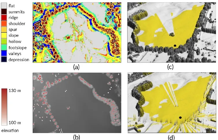
can accurately detect treetops of deciduous and coniferous stands within complex forest structures (Antonello, et al., 2017). We extracted the summits from the classified landform raster map (0.5m resolution) to delineate treetop polygons and used their centroids to designate location and height of the tree trunk. We assumed that the apex of the canopy corresponded with the trunk location on a straight vertical line to the terrain. In addition, given that deciduous trees in our study area had similar sizes, we assumed a diameter of 1m for larger species (Oaks) and a 0.5 m diameter for smaller species. Finally, the segmented trunks were replaced with the deciduous canopies in DSM to acquire the improved surface model (Fig. 2.5, b).
Figure 2.5. Trunk obstruction modeling process and results: (a) geomorphon landform detection results where the summits are shown in brown, (b) the extracted peaks with elevation values, (c) and (d) show the viewshed maps (yellow) computed from a tentative viewpoint (black dot) before and after trunk modeling, respectively.
Computing viewscape metrics
To obtain viewscape metrics, we measured the composition and configuration of viewscapes computed from 342 viewpoints (centroids of a 30 m grid) across the study area (Figure 6).Viewshed was computed on the DSM at the eye-level (1.65 m), and considering maximum visibility range of 3000 meters. We used GRASS GIS viewshed function, which uses a computationally efficient algorithm (line sweeping method) suitable for performing viewshed computation on a high-resolution DSM (Haverkort, et al., 2009; Vukomanovic, et al., 2018). The algorithm calculates line-of-sight for each cell and its intersections with other cells —assuming that two points are visible to each other if their line-of-sight does not
intersect the elevation model.
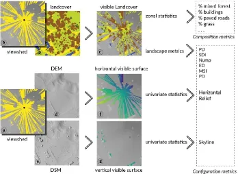
Configuration metrics measure the topological structure of visible surface, as well as spatial arrangement and relationship between different land cover types. They included Total area of viewscape (Extent), Distance to farthest visible feature (Depth), Elevation variability of visible ground surface (Relief), Elevation variability of visible aboveground features (Skyline), Size of visible ground surface (Horizontal), Variability of depth (VdepthVar), Number of patches (NUMP), Shape complexity of patches (MSI and ED), Size of patches (PS), Density of patches (PD), and Land type diversity measured as Shannon’s diversity index (SDI). Depth and Extent were computed directly from the binary viewshed map (visible or non-visible). To compute Horizontal, Relief and Skyline, the viewshed map was
intersected with a bare-earth digital elevation model (DEM) and DSM to develop separate maps of ground (horizontal viewshed) and aboveground (vertical viewshed) visibility, respectively. The rest of variables (Nump, MSI, ED, PS, PD, and SDI) were measured using landscape structure analysis (also called landscape metrics). For more detailed definition, measurement and computation of landscape metrics see Appendix B. The entire GIS analysis and automation workflow was performed via a python script implemented in GRASS GIS.
Immersive Virtual Environment (IVE) Survey of perceived visual characteristics
IVE stimuli
To select viewpoints for model verification we assessed the viewscape metrics using two selection criteria: (1) the visual attributes of the selected viewpoints should approximately represent the range of values of the 342 viewpoints; and (2) viewpoints be at least two grid cells (60m) apart to ensure that they spatially represent the study area. A selection of 24 points satisfied these criteria and were considered for acquiring photographs (See Appendix B for the descriptive statistics of viewscape metrics, and Fig. 2.8 for the panoramic photographs of the selected points).
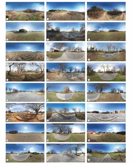
Viewpoints were located using a handheld GPS device (Trimble model, 10-50 cm accuracy). At each location, we took an array of 54 (9 x 6) photographs, at the eye-level (1.65 cm), using a Canon Eos 70D camera fixed on a robotic mount (Gigapan Epic Pro; Fig. 2.7a). All photographs were taken over four days in Feb 2017, in similar weather and lighting conditions. We stitched the images to acquire a 25 Megapixels panoramic image with spherical projection, i.e., equirectangular image (Fig. 2.7b). Through a process known as cube mapping (Dimitrijevic, 2016), each equirectangular image was unfolded into six cube faces (Fig. 2.7c). In virtual reality software, these faces are wrapped as a cubic environment around the viewer (i.e., skybox; Fig. 2.7d).
Figure 2.8. Equirectangular images used in IVE survey. Note: the images have spherical distortion.
Survey Procedure
In total, 100 undergraduate students at a university in the southeastern United States participated in this study. The mean age among the participants was 19.56 years (SD = 3.17); 51% were male (N = 51) and 70% were white (N = 70). Participants’ study background varied; 47% were from parks recreation and tourism management, 25% from sport management and 28% from natural and social sciences.
Participation in the study was voluntary, and those who volunteered were entered in a random drawing for one of the ten $25 gift cards to an online merchant.
Perceived visual characteristics were measured using three items. Visual access (also called visual scale), broadly defined as size, shape, diversity, and degree of openness of landscape rooms or perceptual units was measured using one item without explicit reference to openness: “How well can you see all parts of this environment without having your view blocked or interfered with?” (Herzog, & Kropscott, 2004). The response options ranged from 0 = not at all to 10 = very easy. Naturalness defined as the extent to which landscape is close to a perceived natural state (Dramstad, et al., 2006; Ode, et al., 2009) was measured by a single item “How natural do you perceive this environment?” using a 11-point scale with 0 = not natural, 10 = very natural (Marselle, et al., 2016). For perceived complexity participants responded to the statement “How complex you perceive this environment? “ using a 11-point scale, 0 = not at all, 10 = very complex (Lindal and Hartig, 2013) .
The IVE survey was carried out in a controlled lab environment. Upon participants’ arrival, a researcher assisted them to don and adjust HMD (Oculus CV1), practice rotating around, and interacting with the joystick controller. To familiarize participants with experience of immersion and responding to on-screen survey, they experienced two mockup IVE scenes depicting an urban plaza and a park. For each scene, they responded to three statements measuring perceived realism and presence in the virtual environment. After the warmup phase, each respondent experienced 24 randomly displayed IVEs with a 2-minute recess after the 12th scene. Each of the IVE scenes was to be rated on only one of the response variables (perceived visual access, complexity, and naturalness). The variable for rating was randomly selected by the VR application at the start of the study. The choice of splitting survey questions was guided by a pilot study, in which participants (N = 11) reported a sense of fatigue, boredom and confusion after responding to multiple survey items for each immersive scene.
developed as a python script and executed in World Vizard VR development software (WorldViz Inc, Version 5.4).
Following the experimental session, participants filled-out a brief pen-and-paper survey including questions about age, field of study, ethnicity, and familiarity with the landscapes they experienced. Total duration of each session was on average 40 minutes (range 37- 46). Data were collected over four weeks in March 2016. The study protocol was approved by the university’s Institutional Review Board.
Viewscape model assessment
We used multiple linear regression analysis to test the capacity of the viewscape model to predict each of the three perceived measures (visual access, naturalness, and perceived complexity). A stepwise variable selection based on the minimization of the Akaïke Information Criterion (AIC) was applied to fit the best predictive model for each dependent variable. In cases involving landscape metrics and compositional variables, it is recommended to assess predictors for multicollinearity (Bortz, 1993). Therefore, we filtered out the variables with strong multicollinearity based on the correlation matrix among all factors (see Appendix C). Additionally, for each of the regression models we diagnosed collinearity using the variance inflation factor (VIF) to include variables with tolerance of larger than 0.1 and VIF smaller than 10, as suggested by Hair et al. (2009). The prediction power of regression models are reported using adjusted coefficients of determination (R2
adj), and the relative contribution of each variable to the model is
reported using standardized regression coefficients (Table 2.1).
Results
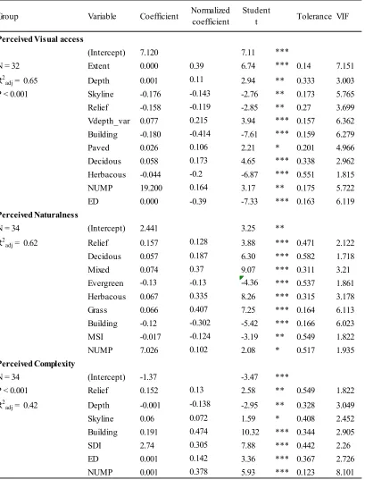
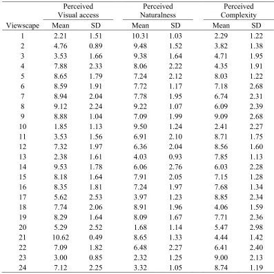
The mean values of perceived visual access of IVEs varied between 1.85 and 10.62 (Table 2.2). Very high values were assigned to viewscape with long vistas and large viewshed areas (scenes 21, 14), and viewscapes enclosed by forests, hills, and buildings (scenes 10, 1, 13) obtained the lowest values. The selected regression model for perceived visual access included 11 variables and produced an adjusted coefficient of determination (R2
adj) of 0.65, P <0.001 (Table 2.1). Extent had the strongest positive
contribution to the model, followed by Viewdepth_var and Depth. Skyline and Relief, respectively, had a negative correlation with perceived visual access. From the compositional metrics, Building had a strong negative impact on perceived visual access, whereas Deciduous and Paved positively contributed to the model. Among configuration metrics, ED (edge density) had a strongest negative contribution to the model, while NUMP (number of patches) was positively related to perceived visual access.
highly built areas with little vegetation coverage received the lowest ratings (scenes 20, 23). With a selection of nine variables, the regression model explained 62% of variation in Perceived naturalness (R2
adj = .62, P <0.001). The majority of variation was explained by compositional metrics. Grass coverage
had the highest positive correlation with perceived naturalness, followed by Mixed, Herbaceous and Deciduous coverage. An inverse significant correlation was found for Buildings. From the configuration metrics, Relief and NUMP had positive contribution, and MSI had negative contribution to the model. Perceptions of complexity varied from 2.29 to 9.9. The lowest values were assigned to viewscapes with lowest SDI (scenes 1 and 10), whereas those with highest SDI were perceived as highly complex. With a selection of seven visual attributes the model explained 42% percent of variation in perceived complexity (R2
adj = .62, P <0.001). Most of the contribution came from configuration variables (Table 2.1). Among
those, NUMP had the highest positive impact, followed by SDI and ED. Relief and Skyline—measures of terrain and above-terrain vertical variability—both positively affected perceived complexity, while Depth had a negative correlation. From the composition metrics, relative Building coverage was the only and the most positively correlated variable with perceived complexity.
Discussion
Table 2.1. Multiple linear regression models for the three visual charactristics, perceived visual access, perceived naturalness, and perceived complexity.
Variables: Vdepth_var = view depth variation, NUMP = patch number, ED = edge density, MSI= mean shape index SDI= shannon diversity index.
Group Variable Coefficient Normalized
coefficient
Student
t Tolerance VIF
Perceived Visual access
(Intercept) 7.120 7.11 ***
N = 32 Extent 0.000 0.39 6.74 *** 0.14 7.151
R2adj = 0.65 Depth 0.001 0.11 2.94 ** 0.333 3.003
P < 0.001 Skyline -0.176 -0.143 -2.76 ** 0.173 5.765
Relief -0.158 -0.119 -2.85 ** 0.27 3.699
Vdepth_var 0.077 0.215 3.94 *** 0.157 6.362
Building -0.180 -0.414 -7.61 *** 0.159 6.279
Paved 0.026 0.106 2.21 * 0.201 4.966
Decidous 0.058 0.173 4.65 *** 0.338 2.962
Herbacous -0.044 -0.2 -6.87 *** 0.551 1.815
NUMP 19.200 0.164 3.17 ** 0.175 5.722
ED 0.000 -0.39 -7.33 *** 0.163 6.119
Perceived Naturalness
N = 34 (Intercept) 2.441 3.25 **
R2
adj = 0.62 Relief 0.157 0.128 3.88 *** 0.471 2.122
Decidous 0.057 0.187 6.30 *** 0.582 1.718
Mixed 0.074 0.37 9.07 *** 0.311 3.21
Evergreen -0.13 -0.13 -4.36 *** 0.537 1.861
Herbacous 0.067 0.335 8.26 *** 0.315 3.178
Grass 0.066 0.407 7.25 *** 0.164 6.113
Building -0.12 -0.302 -5.42 *** 0.166 6.023
MSI -0.017 -0.124 -3.19 ** 0.549 1.822
NUMP 7.026 0.102 2.08 * 0.517 1.935
Perceived Complexity
N = 34 (Intercept) -1.37 -3.47 ***
P < 0.001 Relief 0.152 0.13 2.58 ** 0.549 1.822
R2adj = 0.42 Depth -0.001 -0.138 -2.95 ** 0.328 3.049
Skyline 0.06 0.072 1.59 * 0.408 2.452
Building 0.191 0.474 10.32 *** 0.344 2.905
SDI 2.74 0.305 7.88 *** 0.442 2.26
ED 0.001 0.142 3.36 *** 0.367 2.726
Table 2.2. Mean and standard deviation (SD) of participants ratings of perceived visual access (N = 32), perceived naturalness (N = 34) and perceived complexity (N = 34) of the 24
viewscapes used in the survey
Perceived Visual access Perceived Naturalness Perceived Complexity
Viewscape Mean SD Mean SD Mean SD
1 2.21 1.51 10.31 1.03 2.29 1.22
2 4.76 0.89 9.48 1.52 3.82 1.38
3 3.53 1.66 9.38 1.64 4.71 1.95
4 7.88 2.33 8.06 2.22 4.35 1.91
5 8.65 1.79 7.24 2.12 8.03 1.22
6 8.59 1.91 7.72 1.17 7.18 2.68
7 8.94 2.04 7.78 1.95 6.74 2.31
8 9.12 2.24 9.22 1.07 6.09 2.39
9 8.88 1.04 7.09 1.99 9.09 2.68
10 1.85 1.13 9.50 1.24 2.41 2.27
11 3.53 1.56 6.91 2.10 8.71 1.75
12 7.32 1.97 6.36 2.04 8.56 1.60
13 2.38 1.61 4.03 0.93 7.85 1.13
14 9.53 1.78 6.06 2.76 6.03 2.28
15 8.18 1.64 7.91 2.05 7.15 1.28
16 8.35 1.81 7.24 1.97 7.68 1.34
17 5.62 2.53 3.97 1.23 8.85 2.34
18 7.74 2.06 8.91 1.96 4.06 1.59
19 8.29 1.64 8.09 1.67 7.71 2.36
20 5.29 2.52 1.68 1.14 5.47 2.98
21 10.62 0.49 8.65 1.33 4.44 1.42
22 7.09 1.82 6.48 2.27 6.41 2.40
23 3.00 0.85 2.32 1.25 9.00 2.13
24 7.12 2.25 3.32 1.05 8.74 1.19
Predicting visual characteristics
Statistically, viewscape models provide results with good explanatory power. Regression models explain almost 65% of the variance at best (naturalness, visual access) and as much as 45% at worst (complexity). These results are comparable to those in a similar analysis by Schirpke et al. (2013) and Sahraoui et al. (2016) that estimated perceptions of mountain regions and urban-rural fringes, respectively using viewscapes.
indicating that the observer’s distance between the obscuring elements (depth) and the amount of visible space (extent) have strong influence on perceived visual access (Herzog, & Kropscott, 2004; Stamps, 2010; Tveit, 2009). Depth variation –the spatial variation of the view depth (Sahraoui, Clauzel, et al., 2016)– also showed positive impact on perceived access. This indicator is analogous with “number of perceptual rooms”, which is one the main determinants of visual access, as found by Tveit (2009). An interesting finding concerns the strong negative role of buildings and positive role of deciduous trees in perceived visual accessibility, emphasizing the importance of permeability (porosity) of the obscuring elements. Indeed, in leaf-off season deciduous forests allow for more visibility through the branches compared to evergreen and mixed forests. Similarly, horizontal surfaces occupy a smaller proportion of the visible landscape unlike buildings, whose vertical development leads to significant visual salience. For perceived naturalness, we found a positive role played by green spaces and natural groundcover such as grasslands and herbaceous land cover, which is consistent with what is generally reported in literature. In contrast to previous studies that combined all forest typologies as a single forest land cover (Dramstad, et al., 1996; Sahraoui, Clauzel, et al., 2016; Schirpke, et al., 2016), incorporation of fine-grained land cover enabled our model to discriminate between forest types and revealed perception differences among them. Mixed forests consisting of more than two stand types and abundantly covered by mosses and lichens, were perceived as more natural than the deciduous and evergreen specimens, which parallels previous studies suggesting that less maintained and varied representation of vegetation positively impact perceived naturalness (Ode, et al., 2009; Tveit, et al., 2006). Also, as expected, man-made elements, such as residential or administrative buildings, had a negative effect in naturalness judgments. We also found strong impact of relief indicating that viewscapes with higher vertical variation or rugged terrains were perceived as more natural. Although positive contribution of relief to aesthetic preferences has been confirmed by several studies, there is no prior evidence regarding relationships with perceived naturalness as a basis for comparison.
Also, contrary to our expectations with regard to the literature on landscape visual characteristics (Tveit, et al., 2006), shape index and number of visible patches had positive association with perceived
naturalness. It is generally suggested that a more varied patch shapes may be perceived as more natural compared to a straight edge (Bell, 2001; Ode, et al., 2009) and landscapes consisting of small, fragmented patches may be interpreted as less natural, compared to those with one large woodland patch. We
and “holes” produced by viewshed analysis.
Turning to the perceived complexity model, land cover heterogeneity (SDI), edge density (ED) and number of visible patches (NUMP) had strongest impact, confirming what is generally reported in environmental psychology oriented work suggesting that number (richness) and /or diversity (arrangement) of visible landscape have strong influence on perceived complexity and aesthetic preferences (Berlyne, 1974; Kaplan & Kaplan, 1989; Stamps, 2004). Previous studies using landscape metrics to compute complexity, generally assumed landscape as a planimetric surface and focused on horizontal (land cover) heterogeneity. We dissected the viewscape into surface and above surface
elements to compute two vertical heterogeneity factors, relief and skyline variability – features that play a key role in human perception and preferences. Our results indicate a positive impact of relief on
complexity suggesting that participants perceived rolling terrains more complex than flat ones. Skyline variability was omitted from all three visual characteristic models due to strong collinearity with relief in our study area. This variable deserves further exploration as it reveals the complexity of horizon such as its smoothness and the number of times the horizon is broken, which are shown to impact perceived complexity.
Complexity of the view, as represented by elements distributed in panoramic image, may not be readily transferable to spatial distribution of these elements across a landscape’s surface, even less so as represented in 2D spatial data (Ode, et al., 2010). As such, images may convey additional information such as shape and color of buildings, presence of car and people, even fractal dimension of tree branches all can influence perceived complexity. To supplement this study, it would be instructive to further test the validity of viewscape models by using image-based analysis complexity such as attention-based entropy measures (e.g., Rosenholtz & Nakano, 2007), object counts (e.g., Fairbairn, 2006; Harrie & Stigmar, 2010), image compression algorithms (Palumbo, et al., 2014), landscape metrics analysis (Stamps, 2003), and fractal dimension (Hagerhall, et al., 2008; Stamps, 2003; Taylor, et al., 2005). It should be also observed that a single survey item for complexity might have not reliably captured perception of complexity. Complexity is an intricate and multi-faceted notion and different participants may have interpreted it differently (Schnur, et al., 2018). Recommendation for future analysis include using multiple-item survey, or if not applicable, briefing participants with a distinct definition of complexity to acquire a more homogenous baseline understanding of the concept.
Methodological contributions and consideration
our knowledge, has not been previously incorporated into viewscape models. However, this technique is most effective in leaf-off season where canopy has small impact on visibility, whereas in leaf-on season it may lead to over-estimation of visibility. Also, we assumed a binary occlusion system in which trees either completely obstruct visibility or not at all, whereas in reality tree canopy may not be entirely opaque, depending on the foliage type and density. Alternatively, more nuanced methods such as use of volumetric (voxel-based) 3D visibility models (Chmielewski, & Tompalski, 2017) or calculating vision attenuation based on foliage density and seasonal variation may be preferred (Bartie, et al., 2011). These techniques however, may pose challenges due to prohibitive computing time and limited integration with GIS analysis (Ode, et al., 2010). Another point worth mentioning is that we assumed similar trunk diameters for all the decimated trees given that the majority of the deciduous trees in our study area similar sizes. However, in areas with more varied tree typology, this can potentially cause errors in estimation of under-canopy visibility, especially when the viewpoint is near the trunk. More precise estimation of the trunk can be achieved using tree diameter at breast height (DBH) metric calculated from height (derived from lidar point) and species growth coefficients (Murgoitio, et al., 2017).
An additional contribution of this work includes a novel method for model assessment through IVE technology. Employing IVE images allowed us to capture and display the entire FOV, thereby addressing the concerns regarding the inconsistency of perspective photographs (Ode, et al., 2010) with viewshed coverage, and correspondence with “in-situ” experience (Appleton, & Lovett, 2003). However, photograph based IVEs are static and limit participant’s navigation (moving in the environments) and may include contents that are not captured in the spatial data (e.g., people and cars). Alternatively, 3D simulations and game environments that generate landscape views from geospatial data can be used to achieve higher control over the scene content and implement enhanced interactions (eg., allowing user controlled walk-throughs). However, it can be argued that photorealistic panoramas as a cost-effective and easy, yet highly realistic method to capture viewscapes, runs up against the problem of low ecological validity, and higher production effort of 3D simulations.
Limitations and future work
We should emphasize the need for consideration of more detailed and case-relevant land cover
vegetation, and attributes such as maintained and unmaintained vegetation. These indicators are linked to aesthetic preferences, or important visual characteristics such as imagability and stewardship (Ode, et al., 2009). Thus, a possible avenue to improve explanatory power of viewscape models can be using a more granular classification aligned with indicators established in environmental psychology and landscape visual character literature.
We should note that unrestricted exploration of 360 viewscapes afforded by HMDs may come at a cost of reduced control over the amount of visual information that participants receive from a scene. The extent that participants explore the immersive scene and thus the information they receive, may vary based on their level of engagement, comfortability and familiarity with the VR equipment, and preference to certain elements and characteristics. Also, as opposed to unique perspective of still images, the unconstrained horizontal and vertical viewing generates myriad of perspectives and occlusions, which poses additional standardization challenges. Although we tried to control for these biases by instructing participants to thoroughly explore each IVE scene and base their response on the experience of the place as a “whole”, we cannot make strong inferences of the relative contribution of scene element to
perceptions and whether participants received the same information from each scene. In this respect, it would be interesting to examine whether the viewing patterns play a part in respondents’ perception of immersive scenes and explore specific contribution of certain perspectives or certain landscape elements on perceptions. This can be achieved by leveraging the ability of modern HMDs that record user’s head orientation and eye-movement in real-time, allowing for establishing the links between viewing behavior, viewscape characteristics, and perceptions.
2016).
Conclusion
References
Antonello, A., Franceschi, S., Floreancig, V., Comiti, F., & Tonon, G. (2017). APPLICATION OF A PATTERN RECOGNITION ALGORITHM FOR SINGLE TREE DETECTION FROM LiDAR DATA, XLII(July), 18–22.
Appleton, K., & Lovett, A. (2003). GIS-based visualisation of rural landscapes: Defining “sufficient” realism for environmental decision-making. Landscape and Urban Planning, 65(3), 117–131. Arriaza, M., Cañas-Ortega, J. F., Cañas-Madueño, J. A., & Ruiz-Aviles, P. (2004). Assessing the visual
quality of rural landscapes. Landscape and Urban Planning, 69(1), 115–125.
Barry, S., & Elith, J. (2006). Error and uncertainty in habitat models. Journal of Applied Ecology, 43(3), 413–423.
Bartie, P., Reitsma, F., Kingham, S., & Mills, S. (2011). Incorporating vegetation into visual exposure modelling in urban environments. International Journal of Geographical Information Science, 25(5), 851–868.
Barton, J., Hine, R., & Pretty, J. (2009). The health benefits of walking in greenspaces of high natural and heritage value. Journal of Integrative Environmental Sciences, 6(4), 261–278.
Bell, S. (2001). Landscape pattern, perception and visualisation in the visual management of forests. Landscape and Urban Planning, 54(1–4), 201–211.
Brabyn, L., & Mark, D. M. (2011). Using viewsheds, GIS, and a landscape classification to tag landscape photographs. Applied Geography, 31(3), 1115–1122.
Cavailhès, J., Brossard, T., Foltête, J. C., Hilal, M., Joly, D., Tourneux, F. P., … Wavresky, P. (2009). GIS-Based hedonic pricing of landscape. Environmental and Resource Economics, 44(4), 571– 590.
Chmielewski, S., & Tompalski, P. (2017). Estimating outdoor advertising media visibility with voxel-based approach. Applied Geography, 87, 1–13.
Collado, S., Staats, H., & Sorrel, M. A. (2016). A relational model of perceived restorativeness: Intertwined effects of obligations, familiarity, security and parental supervision. Journal of Environmental Psychology, 48, 24–32.
Çöltekin, A., Lokka, I.-E., & Zahner, M. (2016). On the usability and usefulness of 3D
(geo)visualizations -- A focus on virtual reality environments. ISPRS - International Archives of the Photogrammetry, Remote Sensing and Spatial Information Sciences.
Dias, E., Linde, M., & Scholten, H. J. (2015). Geodesign: integrating geographical sciences and creative design in envisioning a “New Urban Europe.” International Journal of Global Environmental Issues, 14(1/2), 164–174.
Dramstad, W. E., Olson, J. D., & Forman, R. T. T. (1996). Landscape Ecology Principles.pdf. Landscape Ecology.
Gobster, P. H., Nassauer, J. I., Daniel, T. C., & Fry, G. (2007). The shared landscape: What does aesthetics have to do with ecology? Landscape Ecology, 22(7), 959–972.
Hagerhall, C. M., Laike, T., Taylor, R. P., Küller, M., Küller, R., & Martin, T. P. (2008). Investigations of human EEG response to viewing fractal patterns. Perception, 37(10), 1488–1494.
Hair, J. F., Black, W. C., Babin, B. J., & Anderson, R. E. (2009). Multivariate Data Analysis (7th ed.). New Jersey: Pearson.
Haverkort, H., Toma, L., & Zhuang, Y. (2009). Computing visibility on terrains in external memory. Journal of Experimental Algorithmics, 13(1), 1.5.
Herzog, T. R., & Kropscott, L. S. (2004). Legibility, Mystery, and Visual Access as Predictors of Preference and Perceived Danger in Forest Settings without Pathways. Environment and Behavior, 36(5), 659–677.
Hipp, J. A., Gulwadi, G. B., Alves, S., & Sequeira, S. (2015). The Relationship Between Perceived Greenness and Perceived Restorativeness of University Campuses and Student-Reported Quality of Life. Environment and Behavior, (AUGUST), 0013916515598200-.
Jansson, M., Fors, H., Lindgren, T., & Wiström, B. (2013). Perceived personal safety in relation to urban woodland vegetation – A review. Urban Forestry & Urban Greening, 12(2), 127–133.
Jasiewicz, J., & Stepinski, T. F. (2013). Geomorphons-a pattern recognition approach to classification and mapping of landforms. Geomorphology, 182(January 2012), 147–156.
Keane, T. (1990). The Role Of Familiarity In Prairie Landscape Aesthetics. In Proceedings of the 12th North American Prairie Conference (pp. 205–208).
Kim, K., Rosenthal, M. Z., Zielinski, D., & Brady, R. (2012). Comparison of desktop, head mounted display, and six wall fully immersive systems using a stressful task. 2012 IEEE Virtual Reality Workshops (VRW).
Klouček, T., Lagner, O., & Šímová, P. (2015). How does data accuracy influence the reliability of digital viewshed models? A case study with wind turbines. Applied Geography, 64, 46–54.
Kronqvist, A., Jokinen, J., & Rousi, R. (2016). Evaluating the authenticity of virtual environments: Comparison of three devices. Advances in Human-Computer Interaction, 2016.
Kuper, R. (2017). Evaluations of landscape preference, complexity, and coherence for designed digital landscape models. Landscape and Urban Planning, 157, 407–421.
Llobera, M. (2007). Modeling visibility through vegetation. International Journal of Geographical Information Science, 21(7), 799–810.
Marselle, M. R., Irvine, K. N., Lorenzo-Arribas, A., & Warber, S. L. (2016). Does perceived restorativeness mediate the effects of perceived biodiversity and perceived naturalness on emotional well-being following group walks in nature? Journal of Environmental Psychology, 46, 217–232.
Mitášová, H., & Hofierka, J. (1993). Interpolation by Regularized Spline with Tension: II. Application to Terrain Modeling and Surface Geometry Analysis. Math Geol, 25(657).
Moudrý, V., & Šímová, P. (2012). Influence of positional accuracy, sample size and scale on modelling species distributions: A review. International Journal of Geographical Information Science, 26(11), 2083–2095.
Murgoitio, J. J., Shrestha, R., Glenn, N. F., Spaete, L. P., Murgoitio, J. J., Shrestha, R., … Spaete, L. P. (2017). Improved visibility calculations with tree trunk obstruction modeling from aerial LiDAR. International Journal of Geographical Information Science, 27(10), 1865–1883.
Ode, Å., Fry, G., Tveit, M. S., Messager, P., & Miller, D. (2009). Indicators of perceived naturalness as drivers of landscape preference. Journal of Environmental Management, 90(1), 375–383. Ode, Å., Hagerhall, C. M., & Sang, N. (2010). Analysing Visual Landscape Complexity: Theory and
Application. Landscape Research, 35(1), 111–131.
Ode, Å., & Miller, D. (2011). Analysing the relationship between indicators of landscape complexity and preference. Environment and Planning B: Planning and Design, 38(1), 24–38.
Otero Pastor, I., Casermeiro Martínez, M. A., Ezquerra Canalejoa, A., & Esparcia Mariño, P. (2007). Landscape evaluation: Comparison of evaluation methods in a region of Spain. Journal of Environmental Management, 85(1), 204–214.
Palmer, J. F. (2004). Using spatial metrics to predict scenic perception in a changing landscape: Dennis, Massachusetts. Landscape and Urban Planning, 69(2–3), 201–218.
Palmer, J. F., & Hoffman, R. E. (2001). Rating reliability and representation validity in scenic landscape assessments. Landscape and Urban Planning, 54(1–4), 149–161.
Palumbo, L., Makin, A. D. J., & Bertamini, M. (2014). Examining visual complexity and its influence on perceived duration. Journal of Vision, 14(14), 1–18.
Phiri, D., & Morgenroth, J. (2017). Developments in Landsat land cover classification methods: A review. Remote Sensing, 9(9).
Roe, J. J., Ward Thompson, C., Aspinall, P. A., Brewer, M. J., Duff, E. I., Miller, D., … Clow, A. (2013). Green space and stress: Evidence from cortisol measures in deprived urban communities.
International Journal of Environmental Research and Public Health, 10(9), 4086–4103. Sahraoui, Y., Clauzel, C., & Foltête, J.-C. (2016). Spatial modelling of landscape aesthetic potential in
urban-rural fringes. Journal of Environmental Management, 181, 623–636.
Sahraoui, Y., Youssoufi, S., & Foltête, J. C. (2016). A comparison of in situ and GIS landscape metrics for residential satisfaction modeling. Applied Geography, 74(August), 199–210.
Sang, N. (2016). Wild Vistas : Progress in Computational Approaches to ‘ Viewshed ’ Analysis. In S. J. Carver, & S. Fritz (Eds.), Mapping Wilderness (pp. 69–87). Dordrecht: Springer
Science+Business Media.
Schirpke, U., Tasser, E., & Tappeiner, U. (2013). Predicting scenic beauty of mountain regions. Landscape and Urban Planning, 111(1), 1–12.
Schirpke, U., Timmermann, F., Tappeiner, U., & Tasser, E. (2016). Cultural ecosystem services of mountain regions: Modelling the aesthetic value. Ecological Indicators, 69, 78–90.
Schnur, S., Bektaş, K., & Çöltekin, A. (2018). Measured and perceived visual complexity: a comparative study among three online map providers. Cartography and Geographic Information Science, 45(3), 238–254.
Slater, M., Lotto, B., Arnold, M. M., & Sanchez-Vives, M. V. (2009). How we experience immersive virtual environments: The concept of presence and its measurement. Anuario de Psicologia, 40(2), 193–210.
Stamps, A. E. (2003). Advances in visual diversity and entropy. Environment and Planning B: Planning and Design, 30(3), 449–463.
Stamps, A. E. (2010). Effects of Permeability on Perceived Enclosure and Spaciousness, 42, 864–886. Tabrizian, P., Petrasova, A., Harmon, B., Petras, V., Mitasova, H., & Meentemeyer, R. (2016).
Immersive Tangible Geospatial Modeling. In Proceedings of the 24th ACM SIGSPATIAL International Conference on Advances in Geographic Information Systems (p. 88:1--88:4). New York, NY, USA: ACM.
Tang, I.-C., Sullivan, W. C., & Chang, C.-Y. (2015). Perceptual Evaluation of Natural Landscapes: The Role of the Individual Connection to Nature. Environment and Behavior, 47(6), 595–617. Taylor, R. P., Spehar, B., Wise, J. a, Clifford, C. W. G., Newell, B. R., Hagerhall, C. M., … Martin, T. P.
(2005). Perceptual and physiological responses to the visual complexity of fractal patterns. Nonlinear Dynamics, Psychology, and Life Sciences, 9(1), 89–114.
Tveit, M. S. (2009). Indicators of visual scale as predictors of landscape preference; a comparison between groups. Journal of Environmental Management, 90(9), 2882–2888.
Tveit, M. S., Ode, Å., & Fry, G. (2006). Key concepts in a framework for analysing visual landscape character. Landscape Research, 31(June 2015), 229–255.
Uuemaa, E., Antrop, M., Marja, R., Roosaare, J., & Mander, Ü. (2009). Landscape Metrics and Indices : An Overview of Their Use in Landscape Research Imprint / Terms of Use. Living Reviews in Landscape Research, 3, 1–28.
Vukomanovic, J., Singh, K. K., Petrasova, A., & Vogler, J. B. (2018). Not seeing the forest for the trees: Modeling exurban viewscapes with LiDAR. Landscape and Urban Planning, (October), 1–0. Wilson, J., Lindsey, G., & Liu, G. (2008). Viewshed characteristics of urban pedestrian trails,
Indianapolis, Indiana, USA. Journal of Maps, 4(1), 108–118.
CHAPTER 3
Modeling restorative viewscapes: spatial mapping of urban Landscape’s restorative potential using viewscape modeling and photorealistic immersive virtual environments
Preprint
This chapter is a preprint.
Attribution
I performed literature review, carried out the geospatial analysis and survey, processed data, and prepared the manuscript. Perver Baran provided the overall guidance and reviewed the manuscript. Helena