Fitting causal path models to correlation among survey variables

•

•

FITTING CAUSAL PATH MOOELS TO CORRELATIONS AMONG SURVEY VARIABLES

by

Charles Proctor

Institute of Statistics Mimeograph Series NO.·1902

June 1987

*

C. H. Proctor

1. Introduction

Investigators in the social and biological sciences as they attempt to understand the mechanisms that underlie interdependencies among survey

variables, may find themselves doing causal path analysis (Wright, 1968). They will have made measurements on a number of variables for each of a number of cases such as organisms, persons or "systems." Very likely they also will be studying the correlations among these variables. A path analysis consists of specifying a causal path diagram, then calculating estimates of the path coefficients (which are then used to calculate theoretical correlations) and, finally, calculating a measure of fit between the theoretical and the observed correlations.

The causal path diagram is a digraph in which nodes correspond to the variables and directed edges represent their causal connections. A directed edge thus stands for those mechanisms responsible for a corresponding increase

or decrease in level of the terminus variable consequent upon an increase or decrease in level of the origin variable. The path coefficient for an edge is a quantity reflecting the combined strength of the mechanisms. A number of trial diagrams is usually fit and the path coefficients from the most

substantively and statistically adequate one are then interpreted. A

computational routine for the model fitting calculations is the topic of this paper.

*

Written during study leave at the SSRC Data Archive, University of Essex, Colchester, England, 1982.

-•

•

A widely used and widely available program for fitting such models is Joreskog and Sorbom's LISREL (1978). Their program was designed to fit to sample covariances, although it can be used with correlations, while our method was designed from the outset for fitting to correlations. It turns out that

the measure of distance between observed and theoretical correlations used in our program differs from the three distances discussed by Joreskog (1978). Whenever we have compared our results to LISREL's the differences in path coefficients and goodness-of-fit statistic are numerically so slight that

substantive interpretations could not differ. The calculations we describe are simple matrix operations and can thus be programmed with ease in PROC MATRIX of SAS (1979) or with relative ease in FORTRAN. Perhaps their simplicity and the fact they can be used with modest computing equipment is their main advantage.

A listing of the FORTRAN version is available on request. The code is, of course, in working order but since the author is not an accompMished programmer

it is not worth eXhibiting here. This creates problems of exposition. We apologize beforehand for instances where we refer to specific features of the program whose existence the reader must accept on faith.

•

2. Statistical Bases

The program operates on correlations, and thus produces standardized path coefficients rather than metric ones. It sets the variances of latent variables to one, and thus effectively standardizes them as well. It also requires the user to furnish an effective sample size for standard errors and for the

goodness-of-fit chi-square. There are statistical bases behind these features of the computations that researchers should be aware of in deciding how or whether to use them. Let's begin with the question of standardized versus metric coefficients.

A sample of a limited range of observed values (i.e., a small standard deviation) on the causal variable can be expected to show increased

standardized path coefficients but not metric ones. This suggests that metric coefficients are to be preferred. However, the situation is likely to be more

-complex. It is not only truncation or bias in selecting cases, with its effects on variances and also on normality, which can upset path coefficient values. Non1inearities of relationship along with shifts in mean values of the

sample relative to the population could do so. Other distributional features such as skewnesses or variance heterogeneities or, particularly, outliers can

also exercise undue influences on the estimated path coefficients.

The full statistical treatment of these potentially disturbing elements is, in theory, possible. Very roughly speaking, one constructs a likelihood

function for the data with separate parameters to reflect the presence of outliers, degrees of skewness, sizes of means and variances, nonlinearities, heterogeneities of variance, and sizes of path coefficients. If the portion of

correlations, factors from the rest, and if the data seem to accord with this form of function, then one can properly proceed to estimate path coefficients froa the correlations while ignoring the other nuisance features. The fact is that one simply would not expect such a factoring.

In practice we attempt to detect and deal with outliers and to carry out transformations of variables that attain linearity, homogeneous variances and normality of distributions. If the observations are close to multi-normally distributed then means are effectively separated from strengths of

relationships. However, correlations by their definition cannot be separated from variances and thus standardized path coefficients must always be viewed in conjunction with variances. Because, in practice, the correction of outliers and the use of transformations are hardly ever completely effective we would also advocate that path coefficients be viewed in conjunction with means, skewnesses, nonlinearities, variance homogeneities and outliers as well.

Granting, nonetheless, that changes in variances are the more upsetting feature, let's briefly review how one might re-standardize a path coefficient. Suppose there are two estimates of a standardized path coefficient from causal variable j to effect variable i. In one case the standard deviations are s.

1

and s. with p .. as path coefficient and in the other they are s~, s~ with

J lJ 1 J

p~.. We first convert p~ . to a metric coefficient as p~ .s~/s~ and

lJ lJ lJ 1 J

then re-standardize with s. and s. to reach p! .s~s./s~s. which can be

1 J lJ 1 J J 1

compared directly to p ..• For example, if s~

=

s. but s~ • s./2 then twice

lJ 1 1 J J

p~. should be compared to p .. in recognition of the fact that p~. was found

lJ lJ lJ

best be calculated dividing the within clusters degrees of freedom by a design

effect quantity. A study by Kish and Frankel (1970, p. 1070) suggests the

design effect quantity be taken as about 1.5.

Having thus obtained a provisional value of v one should then compute 1/JV

and inquire if this is indeed a reasonable amount of uncertainty to attach to

the observed correlations. If, for example, one calculates correlations from

the whole of the one-in-a-hundred Public Use sample of the U. S. Census, the

value of v could be, say, 4,000,000 in which case 1/JV = .0005. This implies

that, for instance, the value r

=

.315 is not .316 nor .314 and in fact, if

data on the entire U. S. population were used, such an r would with probability

be closer to .315 than to either .316 or .314.

4It

The uncertainties of the observed correlations are here taken to be

effectively summarized by a quantity, say v, the number of degrees of freedom

in each correlation. If the observations are a simple random sample of size n

from the population of interest then v = n-1. If the observations are as a

stratified random sample of sizes n_h from L strata then v =

E~=1nh

- L when

the correlations are computed on the within-stratum sums of squares and cross

products. If the sample of, say, households was drawn in accord with a complex

design with stratification, primary sampling units (PSU) and clusters then

setting v requires considerable judgement.

It is generally wise to subtract stratum means as well as PSU means before

computing correlations. If one can verify that the regression slopes based on

cluster means are not much different from the within-cluster slopes then the

•

However, in interpreting such correlations a researcher would likely feel uneasy asserting such extreme precision. The reason may be that the population of interest for making inferences is one evolving from that of 1980. One tends to discount the 4,000,000 separate individuals and rather visualizes a fewer number of times and of circumstances that they represent. If, for example, he recognizes an uncertainty in an observed r = .32 that easily extends to .31 and

.33 but not so easily to .30 nor .34 then effectively l/~v

=

.02 which suggests v • 250. Such considerations imply that setting v greater than 500 may never be justifiable and even setting v greater than 100 should be done cautiously. 3. Computations

Once having sketched a causal path diagram one can, in completely

mechanical fashion, furnish the corresponding structural equations. The investigator should usually be content to draw the path diagram and let the statistician write the structural equations. The ith such equation appears as

y . •

1

=

1, ••• , P (1 )

where C. represents the set of indexes of observed variables causing i and the

1

set D_i contains indexes of the latent variables causing i. The variates Yl'

Y2' ••• , yp and zp+l' Zp+2' •• ·' zp+q are taken to have unit variances and zero means. The error terms e. are taken to be independent of all else and to have

1

variances determined by the path coefficients n .. and n._k• With latent

lJ 1

variables present there are the additional structural equations:

~ All structural equations can be summarized jointly ;n

8 Y

=

e (3)

where y ;s a column vector containing all p+q var;ab1es and 8 ;s a matrix

with ones on the main diagonal and containing the (negat;ve) path coefficients. All elements of e are taken to be independent so that

where C

=

8-1, provided that 8 ;s nons;ngu1ar which w;ll be the case for any

•

E(e el)

=

D

;s a d;agona1 matrix with ent;res D., say.

J

Not;ce that

y • C e

pract;ca1 example. Thus

R

=

E(y yl) • CDC' ,

(4)

(5)

(6)

where the covariance matrix R also appears to be a correlation matrix due to

the y's having unit variances.

The equations giving the d;agona1 elements of R can be extracted as

1

=

G d , (7)

where 1 ;s a column of ones, d ;s a column vector of the D. arid G

=

(g .. )

J lJ

where g ..

=

C~ . are the squares of the elements of C.

lJ 'J

If one knows the path coefficients, and thus can furnish C, he also can obtain D by solv;ng for the d;agona1 elements as

-1

~ and thereby finds R. That is, R is a fairly simple function of the path coefficients. We will write this function in the form of the vector of

covariance-correlations in the strung-out upper triangle of R, namely as p(8),.

where 8 is the s-component parameter vector of the distinct path coefficient values.

Consider the first m= p(p-1)/2 elements of p, which correspond to the observed correlations, as appearing in, say, P1. Our view of the

corresponding observed correlations, say r₁, is reflected in the following

model equation:

r1 • P1(8) + C • (9)

Although we realize that the distribution of r₁ is quite complex, it is proposed to capture its major features by taking c as multi-normal with a m by m covariance matrix

X.

The (u,v) entry of J is given by

+ PijPjkPjll + PikPjk1\1l + PillPjll1\ll)

2 2 2 2

+ Pi~kll(Pik + Pill + Pjk + Pjll)/2 , (10)

where u is the position of r

ij and v of rkll in the strung out vector r. This expression appears in Pearson and Filon (1898) and is a large sample

approximation to the covariance between r_ij and r kll•

*

Consider that 8 is the true parameter point and 8

r is a parameter point suggested as a trial value.

number, not a correlation.

The SUbscript r refers to an iteration step

* .

When P

(11)

where F_r is the m by s matrix of derivatives of the m entries of P1 with

respect to the s parameters in 8_r, i.e., the Jacobian of the transformation

from 8_r to P

1• It will be supposed that the path diagram is so chosen that Fr has rank s. If the rank is deficient there is a problem of identifiability of

the model.

In earlier versions of the calculations (Proctor, 1978) we patiently

differentiated P

1(8) using calculus and then sUbstituted the entries of 8r into the expressions in order to get Fr. At present we are using the computations

in equations (6), (7) and (8) for producing P1 from 8_r in order to obtain F r numerically. That is, the kth column of F_r is found as:

(12)

where 1_k is a vector of zeroes except for a one in the kth position. We have

used multipliers of a

=

.1, .01 and .001, and the differences in F k were_r,

essentially nil.

Equation (11), the linearized form of equation (9), can be rewritten in the

suggestive form:

and in even more compact notation as:

z

=

X ,. + cS •

(12a)

~

Generalized least squares can be used to estimate

~

giving

(14)

*

However, ~ is a quantity which if added to

e

_r should approach to

e ,

the true value. This leads to the iterative scheme:

(15)

When qr+1 and

e

_r agree sufficiently closely, iteration is stopped.

In accord with the model equation (13) we may take the uncertainties in the estimation of ~ to characterize the uncertainty in

e.

The estimated

covariances of the elements of

e

are the entries of the matrix

(16)

.

In particular the square roots of the diagonal elements of H are standard errors for the parameter estimates.

Goodness of fit is reflected in the distance from observed r

1 to fitted 01 as calculated from

(11)

This observed value of

x

2 may be referred to the theoretical x2 distribution on

m-s degrees of freedom. In view of the tenuousness of the assumptions

In actual calculations we have fit to Fisher's transformation, .5 log (1-r) - .5 10g(1+r), of the correlations. If we replace Z in equations (14), (15) and (17) by: .

U

=

V[.5 log (1 - r) - .5 log (1 + r)] (18)

where V is a diagonal matrix having as entries the reciprocals of the diagonal

entries in ~, then the remainder of the calculations are unchanged.

If the researcher has information on the re1iabilities of certain variables there may be interest in correcting the observed correlations for attenuation. This consists in replacing r .. by K.. r .. where

'J 'J 'J

(19)

If we modify

K•• = 1/.Jr .. r ..

'J " JJ

having entries 'K ..

'J and replace the r .. by the K.. r .. the resulting parameter estimates will fit

'J 'J 'J

to attenuated correlations. A possible difficulty here is the loss of positive in which r .. and r .. are the reliabilities for variables i and j.

" _• JJ

X

by pre- and post-multiplication by the diagonal matrix

•

definiteness in the correlation matrix R upon correction. A suggestion by Fuller and Hidirog10u (1978) is to replace the offending correlation matrix by

the sum of those terms of its spectral decomposition corresponding to positive latent roots. We have not included this replacement step in our programs because we find it is so seldom needed, but it would seem to be a wise provision.

~

equal to the theoretical correlation after each iteration. At the first iteration the missing correlation may be imputed to be equal to the average correlation just to get started. The number of correlations being fit becomes [p(p-')/2-'] or, more generally, [p(p-')/2 - (No. of correlations missing)].

A somewhat more computationally complicated case arises when the researcher wishes to fix some correlation equal to its observed value. This is, I

suspect, the meaning of the common use of double headed arrows in path

,

diagrams. When double headed arrows are placed among the collection of "independent-most" variables they may be more easily represented by the

complete recursive model connections. However, if a double headed arrow occurs between some other pairs of variables then this constitutes a constraint on the

•

parameter vector. A method for obtaining estimates that satisfy the constraint is that of Lagrange multipliers •

Consider fitting equation ('3) where the last ~ components of Z are fixed. The model becomes

Z, • X,_ + 4, , and

(20)

The vector Z, has m-t deviation components and Z2 contains t more to be fixed.

That is, _ is to be found SUbject to the condition X~ • Z2. In such a case one minimizes

(21)

where

(22)

The estimated covariances appear in HM while the calculation of

x

2 is

unchanged. One must also include, in the computer programming approach, a

one-way path plus the constraint to handle each double headed arrow and the degrees

of freedom will then correctly appear as m - s.

Other constraints on the parameter vector that are perhaps of more

practical interest are setting a path coefficient to some specified value, as an

earlier study or a t~eoretical argument may have suggested, or setting one

coefficient equal to some specific multiple of another. The Lagrange

~ multiplier formulation can easily be extended to cover these cases although the computer program as presently written does not include them. One needs· simply

to extend the matrix X₂ and the vector Z2 to include them. If, for example, ~

contained five coefficients and we wished to set the third equal to .5 one

would simply add the element .5 to Z2 and the row (0 0 1 0 0) to

x

2• In order, as a further example, to require the first coefficients to be equal one-third

the second the last row of X

2 is made to be (1 -1/3 0 0 0) and the last element of Z3 is put to zero. In these cases a degree of freedom must be removed for

each constraint since no additional parameter is being introduced.

Programming Considerations for the Interactive Version

A program that was written to do the calculations interactively accepts

nine items of input and furnishes nine items of output. The least amount of

then fit a complete recursive model based on the causal ordering implicit in

the ordering of the variables. That is, all variables cause y" all but y, cause Y2 ' all but y, and Y2 cause Y3' etc. The path coefficients for this complete recursive model are in fact furnished as the first item (item A) of output and they are also used in forming starting values for whatever path model is furnished.

Any digraph having fewer edges than there are observed correlations is a legitimate candidate to be fit. This includes digraphs with loops as well as those having latent variables. If there is a relatively large correlation between two variables, and yet there is no very direct linkage in the digraph between the two, the iterative computations for estimating path coefficients may not converge. This condition will be signalled in the third (or C) item of output which traces the parameter values at each iteration. Path coefficient values ~f -.99 and .99 may also appear. They reflect an attempt to go below or

•

above a reasonable size of path coefficient in order to accommodate to some unrealistic feature of the model.

The path diagram is input as an incidence matrix of zeroes and ones and the user generally needs to prepare this matrix before starting to input his

problem. With P observed and q latent variables the incidence matrix is (p+q) by (p+q). Rows will represent the causal variables and columns the effect variables. For example, the model with Y3 causing Y2 and Y2 causing y,has

incidence matrix:

o ,

0 0 0 ' 0 0 0

e

has incidence matrix: 0 0 0 0 1 0 0 0 0 0 1 0 0 0 .0 0 0 1

0 0 0 0 0 1 0 0 0 0 0 0 0 0 0 0 0 0

After counting the paths, the program queries if all path coefficients are to be treated as separate parameters or if some are to be made equal in groups. If the latter, the user must input another matrix of zeroes and ones to record the equalities of path coefficients. For example, to equate the two path coefficients from each of the latent variables of the previous model, one furnishes the matrix:

1 0 0 0 0 0 1 1

Here columns represent path coefficients and rows represent separate parameters.

•

The program was written in single precision and the criterion for convergence was taken as:

Also, if more than 10 iterations are required the iteration will be stopped. The interactive version allows the user to resume iteration, which he would do if there were none or only a few parameter estimates at -.99 or .99. Sometimes the starting values may be seen to be unrealistic and the user may then choose to change these and try again.

coefficient equalities and this also is the type of marginal modification one may wish to examine. Next up the hierarchy is the path diagram incidence matrix, and then the number of latent variables. Next is degrees of freedom, then fixed correlations, the reliabilities, then observed correlations and, finally (and also firstly) the number of observed variables. Missing

correlations are entered as -5, a code for missingness, and are so detected

among the observed correlations.

We have mentioned items A and C of output. Item B shows the starting

values used. Item 0 contains the goodness of fit or X2 quantity, its degrees of freedom and its level of significance as a tail area of the chi-square distribution. The degrees of freedom are naively calculated as the number of observed and not missing correlations less the number of parameters. In an example to be discussed below there are fewer distinct correlations than observed ones and this illustrates the case when the degrees of freedom may

•

have to be reduced by the knowledgeable user from what the program furnishes. Item E lists the observed correlations, the correlations after attenuation correction and then their theoretical values. In earlier versions of the

program there were also listed chi-square contributions and one may choose to reintroduce these. They were computed as follows. Recall that

2 -1

X

=

(r - p)l~ (r - p) (23)

l ' -1/2

By introducing a, so called, Cholesky decomposition of ~- , namely ~ , this becomes:

~

where c' • (r -

p),~-1/2.

The squares of the elements of c may be called chi-square contributions and, when large, are useful in indicating points of particularly poor fit.

Item F of output lists paths and the estimated path coefficients with their standard errors. Item G lists the variables, their names, their re1iabi1ities, and their residual variances. Item H gives all variances and covariances of the parameter estimates and Item I provides all the theoretical correlations, including those involving latent variables which were missing from item E. Program Performance

If there are no loops in the path diagram, nor are latent variables present and if the error terms in the structural equations (1) are independent of all else and normally distributed, then the maximum likelihood estimates for the

"ij with j e C_i can be seen to be equivalent to the sample regression

coefficients when y. is regressed on just he y. with j e

c ..

This separable

1 J 1

regressions result applies to metric path coefficients but would also seem to be a reasonable procedure for obtaining estimates of standardized path

coefficients from correlations. At any rate, numerical examples suggest that this property is true of the computational scheme and a proof based on the

asymptotic multi-normal distribution of sample covariances among standardized variables should be possible.

A simple example of such a model was cited above in which Y3 causes Y2 and Y2 causes Y1 but no path connects Y3 to Y1. It can be shown algebraically that

the matrix multiplication X,~-1 of (14) for this case produces a 2 by 3

matrix with zero entries in the (1,2) and (2,2) positions so that the value of r

variables would have p-1 paths from y. to y. 1 for i

=

1, ••• , p-1, and the

1 1+

estimates should be

n.

1

=

r. '+1. This result has been found to be true of

1+ 1,1

numerical examples but the proof of its generality remains to be furnished. In order to tax the calculations we input the observed correlations as

r₁₂

=

.4, r₁₃

=

.5 and r₂₃

=

.4 under the single causal chain model. Twenty-six iterations later the stability criterion dropped below 10-7 with estimates

of P12

=

.39992 and P23

=

.40008. The fit statistic was 19.84 on one degree of freedom when n

=

100 had been used as degrees of freedom in each correlation.

An example of path analysis with latent variable, that was discussed by Joreskog and Goldberger (1975), see Fig. 1, can serve here to illustrate the various features of input and output, see Table 1, of the current program as well as to compare its results to theirs. They chose to set the residual

variance of the latent variable equal to one so' it is ~ecessar.y to change scale on all our path coefficients estimates involving Y7. When one creates a

hypothetical variable its variance is obviously at choice but, following

conventions in factor analysis, it would seem more convenient to standardize it to have total variance of unity, the same as for the observed variables. After scaling by using J.74 and 1/J:7.4 , the path coefficients found here are seen to agree with theirs. Their chi-square value was 12.38 but all n

=

530 cases were used while, in accord with earlier discussion, we set v

=

500 and found

2

X

=

11.25.

Table 1. Contents of Input and Output Items for Example From Joreskog and Goldberger (1975).

Items of Input Selected Items of Output

11 • 6 (Six observed variables) 12 • • 36 .21 .1 .156 .158 .265

.284 .192 .324 .176 .136 .226

.304 .305 .344 (Fifteen correlations)

13 • 1 1 1 1 1 1 (Reliabilities equal 1) 14 • 0 (No exactly fitted correlations)

15 • 500 (Judged OF in correlations)

16 • 1 (One latent variable) 17 • 0 0 0 0 0 0 1 0 0 0 0 0 0 1

o

0 0 0 0 0 1 000 0 1 1 0 00000 1 0 0 0 0 0 0 0 0

o

0 0,1 1 1 0 (Incidence matrix)

18

=

9 (Each coefficient is separate parameter)

19

=

0 (Let program furnish start values)

A • ~ .32 .12 -.04 .09 .01 ~ .18

':rtf

.04 .22 ' " ' 0..04 .18@

.23 .23

@

~

1.00 (Complete recursive coeffic ts with ' residual variances circled)

o •

11.25 (X2 ), 6 (OF), .081 (PO)

F ••47 ± .05, .73 ± .05, .40 ± .05, .23 ± .04, .23 ± .04, .34± .04, .23 ± .06, .10 ± .06, .33 ± .06 (Path coefficients with standard errors for 9 paths)

G

=

.78 .46 .83 .86 .88 1.00 .74 (Residual variances for seven variables)

The next example is of a degree of complexity common to applications. It is based on correlations used in a study (A. H. Halsey, T. F. Heath and J. M. Ridge, 1980) on "education as a channel of social selection." There were seven observed variables: y,. Respondent's Exam Success, Y2

=

Respondent's School

Leaving Age, Y3= Respondent's Secondary School Category, Y4

=

Brother's

Secondary School Category, Y5 • Respondent's IQ, Y6

=

Brother's IQ and

___

---,

Figure 2. Schooling Attainment Process in Britain: Seven observed and one latent variables with 15 paths.

The 21 correlations among the seven variables as Hsted to be input appear

e

as: .745 •652 .417

.

-5 -5 .426 .647 .413 .494 -5 .459 .548 .601 -5 .442 -5 .601 .436 .520 •375 .375 • There are 16 correlations or data

points being fit and thus there are 16 initial degrees of freedom. Three of

these will be exactly fit by the three complete recursive model coefficients of

paths 11, 12 and 13 (see Figure 2) so they may be ignored. Notice the

duplicate value .601 which shows that there are actually 12 correlations, not

13

=

16-3, being fit by the paths in Figure 2 ignoring paths 11, 12 and 13.

The remaining 12 paths include, however, three pairs with the same path

coefficient value. This is due to the symmetry of respondent.to his brother.

That is, paths 7 and 9 are paired and so are paths 8 and 10, as well as paths

14 and 15. Finally, the 12 correlations will be fit by 9 parameters and thus

the chi-square statistic of fit,

x

2

=

9.47, has 3 degrees of freedom. The computer program will show 4 because it cannot, at present, account for the

duplicated value among the correlations to be exactly fit. The path

Table 2. Estimated Path Coefficients and Standard Errors for Process of Schooling Attainment in Britain.

Path Origin Terminum Estimate Std. Error

1 2 1 .5650 .0547

2 7 1 .0589 .0519

3 8 1 2679 .0606

4 3 2 4299 .0811

5 7 2 1978 .0581

6 8 2 1772 .0870

7 7 3 1750 .0416

8 8 3 6559 .0395

9 7 4 .1750 .0416

10 8 4 .6559 .0395

14 5 8 .5336 .0212

15 6 8 .5366 .0212

A major substantive issue to be answered by these data is the relative

effect of Family Material Circumstances versus Family Culture on the

educational attainment variables. The latent variable herein used to represent

Family Culture is viewed as arising from the IQ level evidenced by the children

in the family and is taken to be orthogonal to material circumstances. In

comparing the two sources the relevant path coefficients from Table 2 have been

collected into Table 3.

Table 3. Path Coefficients Giving Strength of Direct Causality, with Standard Errors in Parentheses

Causal Variable

Effect Variable

3. Category of Secondary School 1

=

non selective, 2

=

technical 3

=

grammar, 4

=

independent or

Direct Grant

2. School Leaving Age

1. Exam Success Score

1

=

One or more O-levels,

o

=

Otherwise

~

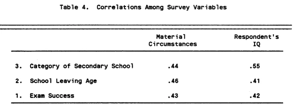
In settling on Category of Secondary School (Y3) the IQ emphasis is impressive although there is very appreciable influence of Material

Circumstances. The two sources of influence seem balanced in their influence on School Leaving Age. Finally, the IQ emphasis appears to be paramount in its influence on Exam Success while Material Circumstances may well be absent in its direct effect.

In their report, which obviously used a different model from ours, the authors state:

"we

have, then, reached an important conclusion, the British educational system has been much less meritocratic than has usually been supposed; IQ is a relatively unimportant determi-nant of the type of school one goes to or of the length of one's school career."

In their model the latent variable reflecting family climate for IQ was placed prior causally to the IQ scores of Respondent's and Brother's. However, in such a model this latent variable would not reflect climate so much as family genetic background unless environment does indeed largely determine IQ and that seems doubtful. The actual meaning of their latent variable was further

clouded by their assignment of a correlation of .3 between it and Material

Circumstances.

One should have considerable reluctance in entering rival interpretations and findings when they are based on estimated path coefficients involving differently located latent variables. The basic evidence remains the

of path coefficients in Table 3. Admittedly the picture is incomplete but the intrusion of IQ into educational attainment seems to be equally as prominent as that of Material Circumstances.

Table 4. Correlations Among Survey Variables

Material Respondent's

Circumstances IQ

3. Category of Secondary School .44 .55

2. SChool Leaving Age .46 .41

1- Exam Success .43 .42

e

References

Fuller, Wayne A., and Hidiroglou, Michael A. 1978. "Regression Estimation After Correcting for Attenuation," Journal of the American Statistical Association 73:99-104.

Halsey, A. H., Heath, T. F. and Ridge, J. M. 1980. Origins and Destinations: Family, Class and Education in Modern Britain, Oxford, England, Claredon Press.

Joreskog, Karl G. 1978. "Structural Analysis of Covariance and Correlation Matrices," Psychometrika 43:443-477.

Joreskog, Karl G. and Goldberger, Arthur J. 1975. "Estimation of a Model with MUltiple Indicators and Multiple Causes of a Single Latent Variable,"

Journal of the American Statistical Association 10:631-639.

Joreskog, K. G. and Sorbom, D. 1978. LISREL IV, User's Guide. Chicago, National Educational Resources.

..

Pearson, Karl and Filon, L. N. G. 1898. "Mathematical Contributions to the Theory of Evolution - IV on the Probable Errors of Frequency Constants and on the Influence of Random Selection on Variation and Correlation,"

Phi7osophical Transactions of the Royal Society, Series A, 191 :229-311. Proctor, Charles. 1978. "Model Fitting to Correlations by Nonlinear

Generalized Least Squares," Abstract 161-34, INS BUl1etin, 1:82-83.

SAS User's Guide, 1919 Edition, Cary, NC, SAS Institute, Inc.