ABSTRACT
KRESS, JEREMY GIFFORD. An Investigation into Soil-Structure Interaction Problems using Discrete Element Method. (Under the direction of Dr. T. Matthew Evans.)
The purpose of this work is to investigate new techniques for predicting behavior in Soil-Structure Interaction (SSI) problems. The response of soil under a given load may be described by interface micromechanics. The approach selected for this study is the discrete element method (DEM). In order to apply this method to typical SSI problems the bulk material parameters of the granular assembly are estimated. One way to determine this information is via strength test simulations such as biaxial compression. Biaxial compression tests performed in this study estimate internal friction angle, elastic modulus, and Poisson‟s ratio within the expected in-situ range for dense sand. Specifically, internal friction angle is computed as 26.6° for critical state and 32.5° for peak state. The elastic modulus is computed over an initial strain range and varies from approximately 12MPa to 25MPa for a series of confining stress levels. In this study the 12MPa value is used for comparison to analytical solutions as it is the worst case modulus producing the largest strains. Also the Poisson‟s ratio is computed to be 0.36 for all confining stress levels.
An Investigation into Soil-Structure Interaction Problems using Discrete Element Method
by
Jeremy Gifford Kress
A thesis submitted to the Graduate Faculty of North Carolina State University
in partial fulfillment of the requirements for the Degree of
Master of Science
Civil Engineering
Raleigh, North Carolina
2011
APPROVED BY:
____________________________ ____________________________ Dr. Mohammed A. Gabr Dr. M. Shamimur Rahman
____________________________ Dr. T. Matthew Evans
ii BIOGRAPHY
iii TABLE OF CONTENTS
LIST OF TABLES ... ix
LIST OF FIGURES ... x
1. INTRODUCTION ... 1
1.1 Introduction ... 1
2. LITERATURE REVIEW ... 4
2.1 Introduction ... 4
2.2 Interface Shear ... 5
2.2.1 Interface Surface Roughness...5
2.2.2 Interface Shear Test Comparisons and Test Simulations ...13
2.3 Shallow Foundations ... 21
2.3.1 Bearing Capacity ...21
2.3.2 Improvements to the Bearing Capacity Equation ...24
2.3.3 Settlement ...26
2.3.4 Model Testing ...29
2.3.5 Induced Stress ...32
2.3.6 Numerical Methods ...32
iv
2.4.1 Pile Installation ...35
2.4.2 Load-Deformation...36
2.4.3 Bearing Capacity ...36
2.4.4 Field Testing ...44
2.4.5 Numerical Methods ...45
2.5 Rigid Retaining Walls ... 49
2.5.1 Earth Pressure Theory ...49
2.5.2 Wall Displacement ...56
2.5.3 Numerical Methods ...56
2.6 Discrete Element Method ... 58
2.6.1 Overview ...58
2.6.2 Strength Testing ...60
2.6.3 Soil-Structure Interaction ...66
2.7 Lunar Regolith... 68
2.7.1 Overview and Characterization ...68
2.7.2 In-Situ Tests ...71
2.7.3 Laboratory Tests ...73
v
3. SHEAR STRENGTH OF GRANULAR MATERIALS ... 76
3.1 Introduction ... 76
3.2 Material Properties ... 77
3.3 Grain Size Distribution & Grain Shape... 78
3.4 Scale Size ... 81
3.5 Biaxial Compression ... 84
3.5.1 DEM Simulation ...84
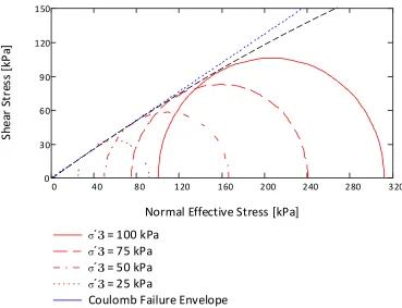
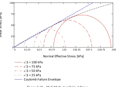
3.5.2 Mohr-Coulomb Peak & Residual Envelope ...86
3.5.3 Elastic Modulus ...93
3.5.4 Poisson‟s Ratio...97
3.6 Interface Shear Strength ... 100
3.6.1 DEM Interface Test...100
4. SOIL-STRUCTURE INTERACTION MODELS ... 107
4.1 Introduction ... 107
4.2 Shallow Foundations ... 109
4.2.1 Assembly...109
4.2.2 Parametric Analyses...110
vi
4.2.4 Particle Rotations ...116
4.2.5 Force Chains ...121
4.2.6 Local Stress Tensors ...124
4.3 Deep Foundations ... 125
4.3.1 Assembly...125
4.3.2 Parametric Analyses...127
4.3.3 Load-Displacement ...129
4.3.4 Particle Rotations ...134
4.3.5 Force Chains ...140
4.3.6 Local Stress Tensors ...141
4.3.7 Additional Measurement Field ...144
4.4 Deep Foundation – Lateral Loading ... 145
4.4.1 Assembly...145
4.4.2 Load-Displacement ...146
4.4.3 Particle Rotations ...149
4.4.4 Force Chains ...150
4.4.5 Local Stress Tensors ...152
vii
4.5 Rigid Retaining Wall ... 156
4.5.1 Earth Stress ...156
4.5.2 Particle Rotations ...164
4.5.3 Force Chains ...166
4.5.4 Local Stress Tensors ...167
5. INTERPRETATION OF RESULTS ... 168
5.1 Introduction ... 168
5.2 Shallow Foundation... 169
5.3 Deep Foundation ... 177
5.4 Laterally Loaded Pile ... 185
5.5 Rigid Retaining Wall ... 189
6. CONCLUSIONS AND RECOMMENDATIONS ... 206
6.1 Conclusions ... 206
6.1.1 Biaxial Compression Test ...206
6.1.2 Interface Shear Test ...207
6.1.3 Shallow Foundation ...208
6.1.4 Deep Foundation Vertical Loading ...209
viii
6.1.6 Rigid Retaining Wall ...210
6.2 Recommendations for Future Work ... 211
REFERENCES ... 213
APPENDIX ... 230
A.1 Rigid Retaining Wall Measurement Fields ... 231
A.2 Rigid Retaining Wall Force Chains ... 236
ix LIST OF TABLES
Table 3.1 - DEM Material Properties (after Evans & Frost, 2008) ... 77
Table 3.2 - Scaling Values of Model Dimensions and Grain Size (after Zhao and Evans 2009) ... 83
Table 3.3 - Friction Value for Confining Stress Cases ... 88
Table 4.4 - Shallow Foundation Parametric Analysis ... 110
Table 4.5 - Deep Foundation Parametric Analysis ... 127
Table 4.6 – Rigid Retaining Wall Parametric Analysis ... 156
Table 4.7 - Movement Required to Mobilize Active and Passive Earth Pressure (after Salgado, 2008) ... 157
Table 5.8 – Deep Foundation Wall Friction Effect on Ultimate Load ... 184
Table 5.9 – At Rest Backfill Pressure Distribution Along Rigid Retaining Wall ... 196
Table 5.10 – Active Case Analytical Versus DEM Results... 204
x LIST OF FIGURES
Figure 2.1 – Coulomb Derivation of Earth Pressure Coefficient (After Bowles 1996) ... 53
Figure 2.2 - Rankine Derivation of Earth Pressure Coefficient (After Budhu 2008) ... 54
Figure 3.3 - GSD used in the DEM assembly ... 79
Figure 3.4 - Grain Aspect Ratio ... 80
Figure 3.5 - Biaxial Compression Assembly & Porosity Field At 7% Axial Strain (From Left to Right, Respectively) ... 85
Figure 3.6 – BC Grain Rotations At 10% Stress (From Left to Right: 25kPa, 50kPa, 75kPa, 100kPa) ... 86
Figure 3.7 - Biaxial Compression Deviator Stress... 87
Figure 3.8 - Void Ratio & Confining Stress for Contractive and Dilative Sands (Salgado 2008) ... 89
Figure 3.9 – M-C Method at Peak Stress ... 90
Figure 3.10 – M-C Method at Critical Stress ... 91
Figure 3.11 – Principle Effective Stress Ratio ... 92
Figure 3.12 - Biaxial Compression Young's Modulus ... 94
Figure 3.13 – Initial Elastic Region of the Deviator Strain Curve ... 95
Figure 3.14 – Small Strain Region of the Deviator Strain Curve ... 96
Figure 3.15 - Biaxial Compression Volumetric Strain ... 98
Figure 3.16 - Biaxial Compression Volumetric Strain ... 99
xi
Figure 3.18 - Interface Surface Roughness & Normal Force Resultants ... 101
Figure 3.19 - Rotations Color Bar for Rotations Figures (deg) ... 101
Figure 3.20 – DEM Interface Shear Test: Region of Shear Localization Developed during Loading ... 101
Figure 3.21 - Definition of Coefficient of Friction (after Uesugi & Kishida 1986b) ... 102
Figure 3.22 - Coefficient of Friction for DEM Simulation and Experimental Results (after Uesugi & Kishida 1986b) (From top to bottom, respectively) ... 104
Figure 3.23 – DEM Interface Shear Results for Friction Angle ... 106
Figure 4.24 - Shallow Foundation Baseline Assembly ... 109
Figure 4.25 - Shallow Foundation Extended Width Assembly ... 111
Figure 4.26 - Shallow Foundation Extended Height Assembly ... 111
Figure 4.27 – Shallow Foundation Model Dimensions Total Resistance ... 113
Figure 4.28 - Shallow Foundation Friction Total Resistance ... 114
Figure 4.29 – Shallow Foundation Base versus Side Wall Resistance ... 115
Figure 4.30 - Rotations Color Bar for Rotations Figures (deg) ... 116
Figure 4.31 - Shallow Foundation Grain Rotations Baseline Case at 0.05B, 0.10B, and 0.20B Vertical Displacements (From Top to Bottom Respectively) ... 117
Figure 4.32 - Shallow Foundation Grain Rotations Extended Height at 0.025B, 0.05B, and 0.10B Vertical Displacements (From Left to Right Respectively) ... 118
xii Figure 4.34 - Shallow Foundation Grain Rotations Extended Width at 0.025B, 0.05B, and
0.10B Vertical Displacements (From Top to Bottom Respectively) ... 120
Figure 4.35 - Shallow Foundation Grain Rotations Extended Width at 0.10B, 0.15B, and 0.20B Vertical Displacements (From Top to Bottom Respectively) ... 121
Figure 4.36 - Shallow Foundation Force Chains at Baseline, Extended Height, and Extended Width Model Size (From Top to Bottom Respectively). Vertical Displacements are 0.20B for all cases shown. ... 123
Figure 4.37 - Shallow Foundation Baseline Vertical Stress at 0.10B (Units: Pa) ... 124
Figure 4.38 - Shallow Foundation Baseline Lateral Stress at 0.10B (Units: Pa) ... 124
Figure 4.39 - Shallow Foundation Baseline Shear Stress at 0.10B (Units: Pa) ... 125
Figure 4.40 – Deep Foundation Baseline Assembly ... 126
Figure 4.41 - Deep Foundation Extended Width Assembly ... 128
Figure 4.42 - Deep Foundation Extended Height Assembly ... 129
Figure 4.43 – Deep Foundation Model Dimensions Total Resistance ... 131
Figure 4.44 - Deep Foundation Friction Total Resistance ... 132
Figure 4.45 - Deep Foundation Toe versus Side Resistance ... 133
Figure 4.46 - Rotations Color Bar for Rotations Figures (deg) ... 134
Figure 4.47 – Deep Foundation Grain Rotations Baseline Case at 0.05B, 0.10B, and 0.20B Vertical Displacements (From Top to Bottom Respectively) ... 135
xiii Figure 4.49 - Deep Foundation Grain Rotations Extended Height at 0.10B, 0.15B, and
0.20B Vertical Displacements (From Left to Right Respectively) ... 136
Figure 4.50 - Deep Foundation Grain Rotations Extended Width at 0.025B, 0.05B, and 0.10B Vertical Displacements (From Top to Bottom Respectively) ... 138
Figure 4.51 - Deep Foundation Grain Rotations Extended Width at 0.10B, 0.15B, and 0.20B Vertical Displacements (From Top to Bottom Respectively) ... 139
Figure 4.52 - Deep Foundation Force Chains at Baseline, Extended Height, and Extended Width Model Size (CW From Top Left Respectively). Vertical Displacements are 0.20B for all cases shown. ... 140
Figure 4.53 - Deep Foundation Baseline Vertical Stress at 0.10B (Units: Pa) ... 141
Figure 4.54 - Deep Foundation Baseline Lateral Stress at 0.10B (Units: Pa) ... 142
Figure 4.55 - Deep Foundation Baseline Shear Stress at 0.10B (Units: Pa) ... 143
Figure 4.56 - Deep Foundation Baseline Coordination Number at 0.10B... 144
Figure 4.57 – Deep Foundation Lateral Loading Assembly at 0.1B Pile Rotation ... 146
Figure 4.58 – Deep Foundation Lateral Loading Lateral Stresses on Foundation Wall . 147 Figure 4.59 – Deep Foundation Lateral Loading Vertical Stresses on Foundation Wall 148 Figure 4.60 - Rotations Color Bar for Rotations Figures (deg) ... 149
Figure 4.61 – Deep Foundation Lateral Loading Grain Rotations at 0.1B Pile Rotation 149 Figure 4.62 - Deep Foundation Lateral Loading Force Chains at 0.1B Pile Rotation .... 151
xiv Figure 4.64 - Deep Foundation Lateral Loading Lateral Stress at 0.1B Pile Rotation
(Units: Pa) ... 153
Figure 4.65 - Deep Foundation Lateral Loading Shear Stress at 0.1B Pile Rotation (Units: Pa) ... 153
Figure 4.66 - Deep Foundation Lateral Loading Coordination Number at 0.1B Pile Rotation ... 155
Figure 4.67 – Rigid Retaining Wall Baseline, Extended Height, and Extended Width (From Top to Bottom Respectively) After Assembly Prior to Loading ... 158
Figure 4.68- Rigid Retaining Wall Load-Displacement Active Case ... 159
Figure 4.69 - Rigid Retaining Wall Load-Displacement Model Size Active Case ... 160
Figure 4.70 - Rigid Retaining Wall Load-Displacement Loading Rate Active Case ... 161
Figure 4.71 - Rigid Retaining Wall Load-Displacement Passive Case ... 162
Figure 4.72 - Rigid Retaining Wall Load-Displacement Model Size Passive Case ... 163
Figure 4.73 - Rigid Retaining Wall Load-Displacement Loading Rate Passive Case .... 164
Figure 4.74 - Rotations Color Bar for Rotations Figures (deg) ... 164
Figure 4.75 - Rigid Retaining Wall Active Baseline, Extended Height, and Extended Width Cases at 0.15 m Lateral Displacement (CW from Top Left Respectively) ... 165
xv Figure 5.77 – Shallow Foundation DEM Simulation Load Curves For all Parametric
Cases ... 170
Figure 5.78 – Definition of QL2 (After Akbas and Kulhawy 2009a) ... 174
Figure 5.79 – Shallow Foundation Normalized DEM & Hyperbolic Fit ... 175
Figure 5.80 – Shallow Foundation Results Summary ... 176
Figure 5.81 - Grain Rotations Shallow Foundation Baseline at 0.20B Vertical Displacement... 177
Figure 5.82 - Deep Foundation DEM Simulation Load Curves For all Parametric Cases ... 178
Figure 5.83 - Deep Foundation DEM Simulation Load Curves ... 180
Figure 5.84 - Deep Foundation Wall Friction Effect on Ultimate Load ... 185
Figure 5.85 - Deep Foundation Laterally Loaded Pile Rotation ... 186
Figure 5.86 - Deep Foundation Laterally Loaded Pile Rotation Results ... 187
Figure 5.87 - Deep Foundation Laterally Loaded Pile Rotation Measurement ... 188
Figure 5.88 - Rigid Retaining Wall Lateral Force Active and Passive Case (From Left to Right Respectively) ... 190
Figure 5.89 - Rigid Retaining Wall Normalized Lateral Force Active and Passive Case (From Left to Right Respectively) ... 190
xvi Figure 5.91 - Rigid Retaining Wall Passive Case Model Dimensions and Loading Rate
(From Left to Right Respectively) ... 192 Figure 5.92 – Wall friction effect on Active and Passive Earth Pressure Coefficient .... 193 Figure 5.93 – At Rest Backfill Pressure Distribution along Rigid Retaining Wall for
distances 2.0m, 1.0m, 0.1m, and 0.05m from the Wall (CW from Top Left,
Respectively)... 195 Figure 5.94 – Grain Rotations Active Case Baseline at 0.15 m lateral displacement .... 196 Figure 5.95 – Grain Rotations Active Case Extended Width at 0.15 m lateral
displacement ... 197 Figure 5.96 – Grain Rotations Active Case Extended Height at 0.15 m lateral
displacement ... 197 Figure 5.97 – Grain Rotations Active Case Slow Loading at 0.15 m lateral displacement
... 198 Figure 5.98 – Grain Rotations Active Case Fast Loading at 0.15 m lateral displacement
... 198 Figure 5.99 – Grain Rotations Passive Case Baseline at 0.20 m lateral displacement ... 199 Figure 5.100 – Grain Rotations Passive Case Extended Width at 0.20 m lateral
displacement ... 199 Figure 5.101 – Grain Rotations Passive Case Extended Height at 0.20 m lateral
xvii Figure 5.102 – Grain Rotations Passive Case Slow Loading at 0.20 m lateral
displacement ... 200 Figure 5.103 – Grain Rotations Passive Case Fast Loading at 0.20 m lateral displacement
... 200 Figure 5.104 – Coefficient of Lateral Earth Pressure during Loading ... 202 Figure 5.105 – Mohr-Coulomb Method for Rigid Retaining Wall ... 203 Figure A.106 - Rigid Retaining Wall Active Baseline Coordination Number at 0.05 m
lateral displacement ... 231 Figure A.107 - Rigid Retaining Wall Active Baseline Lateral Strain at 0.10 m lateral
displacement ... 231 Figure A.108 - Rigid Retaining Wall Active Extended Width Coordination Number at
0.15 m lateral displacement ... 231 Figure A.109 - Rigid Retaining Wall Active Extended Width Lateral Strain at 0.20 m
lateral displacement ... 232 Figure A.110 - Rigid Retaining Wall Active Extended Width Shear Strain at 0.15 m
lateral displacement ... 232 Figure A.111 - Rigid Retaining Wall Active Extended Width Shear Strain at 0.20 m
lateral displacement ... 232 Figure A.112 - Rigid Retaining Wall Active Extended Width Vertical Strain at 0.15 m
xviii Figure A.113 - Rigid Retaining Wall Active Extended Width Vertical Strain at 0.20 m
lateral displacement ... 233 Figure A.114 - Rigid Retaining Wall Active 0.31 Friction Coordination Number at 0.05
m lateral displacement ... 233 Figure A.115 - Rigid Retaining Wall Active 0.31 Friction Lateral Strain at 0.05 m lateral
displacement ... 233 Figure A.116 - Rigid Retaining Wall Active 0.31 Friction Lateral Strain at 0.10 m lateral
displacement ... 234 Figure A.117 - Rigid Retaining Wall Active Slow Loading Lateral Strain at 0.20 m lateral displacement ... 234 Figure A.118 - Rigid Retaining Wall Active Slow Loading Shear Strain at 0.20 m lateral
displacement ... 234 Figure A.119 - Rigid Retaining Wall Passive Fast Loading Vertical Strain at 0.15 m
lateral displacement ... 235 Figure A.120 - Rigid Retaining Wall Passive Fast Loading Lateral Strain at 0.15 m lateral displacement ... 235 Figure A.121 - Rigid Retaining Wall Passive Fast Loading Shear Strain at 0.15 m lateral
displacement ... 235 Figure A.122 – Rigid Retaining Wall Active Force Chains (0.005 scale thickness) at
xix Figure A.123 – Rigid Retaining Wall Active Force Chains (0.005 scale thickness) at
Baseline, Slow Loading, and Fast Loading (CW From Top Left Respectively). Retaining Wall Lateral Displacement is 0.10 m. ... 237 Figure A.124 – Rigid Retaining Wall Passive Force Chains (0.005 scale thickness) at
Baseline, Extended Height, and Extended Width Model Size (From Top to
Bottom Respectively). Retaining Wall Lateral Displacement is 0.10 m. ... 238 Figure A.125 – Rigid Retaining Wall Passive Force Chains (0.005 scale thickness) at
Baseline, Slow Loading, and Fast Loading (CW From Top Left Respectively). Retaining Wall Lateral Displacement is 0.10 m. ... 239 Figure A.126 - Rigid Retaining Wall Active Baseline Case at 0.05 m, 0.10 m, and 0.15 m
Lateral Displacements (From Top to Bottom Respectively) ... 240 Figure A.127 - Rigid Retaining Wall Active Extended Height Case at 0.10 m, 0.20 m,
0.25 m, and 0.30 m Lateral Displacements (CW From Top Left Respectively) 241 Figure A.128 - Rigid Retaining Wall Active Extended Width Case at 0.10 m, 0.15 m, and
0.20 m Lateral Displacements (From Top to Bottom Respectively) ... 242 Figure A.129 - Rigid Retaining Wall Active Wall Friction 0.31 at 0.05 m, 0.10 m, and
0.15 m Lateral Displacements (From Top to Bottom Respectively) ... 243 Figure A.130 - Rigid Retaining Wall Active Slow Loading at 0.10 m, 0.15 m, and 0.20 m
Lateral Displacements (From Top to Bottom Respectively) ... 244 Figure A.131 - Rigid Retaining Wall Active Fast Loading at 0.06 m, 0.10 m, and 0.16 m
xx Figure A.132 - Rigid Retaining Wall Passive Baseline Case at 0.10 m, 0.15 m, and 0.20
m Lateral Displacements (From Top to Bottom Respectively) ... 246 Figure A.133 - Rigid Retaining Wall Passive Extended Height Case at 0.10 m, 0.15 m,
and 0.20 m Lateral Displacements (CW From Top Left Respectively) ... 247 Figure A.134 - Rigid Retaining Wall Passive Extended Width Case at 0.10 m, 0.15 m,
and 0.20 m Lateral Displacements (From Top to Bottom Respectively) ... 248 Figure A.135 - Rigid Retaining Wall Active Wall Friction 0.31 at 0.10 m, 0.15 m, and
0.20 m Lateral Displacements (From Top to Bottom Respectively) ... 249 Figure A.136 - Rigid Retaining Wall Active Slow Loading at 0.10 m, 0.15 m, and 0.20 m
Lateral Displacements (From Top to Bottom Respectively) ... 250 Figure A.137 - Rigid Retaining Wall Active Fast Loading at 0.10 m, 0.15 m, and 0.20 m
1
1. INTRODUCTION
1.1 Introduction
Basic material properties of foundations such as surface roughness and surface geometry control a great deal of the behavior of adjacent soil mass during loading. From simple shear lab tests Uesugi and Kishida (1986a) show that for several dry sand types the failure mechanism begins along the foundation surface at low roughness and moves to the soil mass at high roughness. Jensen (1999) showed that a simple interface shear test could be modeled in two dimensions using DEM. During initial studies, simple geometry (i.e., sawtooth) proved sufficient to capture the basic effect of foundation surface roughness. Results described herein show that the interface shear test using DEM reasonably captures experimental results of Uesugi and Kishida (1986a). Hence this approach proves to be an attractive means to further develop soil structure interaction models to predict soil response. These models are especially useful in, for example, an extraterrestrial environment, where local conditions are not readily reproducible and load testing is unreasonable. Throughout the development of DEM one recurring problem is encountered: excessive particle rotations, as described by Bardet (1994). A simple solution pursued by many investigators is the definition of particle clumps or groups which not only reduce excessive rotations, but also capture more realistic grain geometry.
2 via numerical strength tests, specifically biaxial compression tests. Biaxial compression tests are shown herein to predict internal friction angle, elastic modulus, and Poisson‟s ratio within expected ranges for dense sand. In order to reduce computational cost, the two dimensional DEM model is employed which acts in only one particle unit in the third dimension. This dimension length is taken to be D50 to for comparison with analytical
solutions.
The typical simulation process for generating and loading the DEM simulation involves assembly of the grain space within predesigned model walls, consolidation and decompression of the granular assembly, installation of foundation structure, additional cycling and instructions, and the final step of loading and deformation of the model. Loading is typically halted when the grain rotations show that major shear bands have developed and reached critical state. Finally soil response is measured and results are saved. Note that before final results of the DEM simulation may be run for SSI cases an extensive parametric analysis is made to evaluate the effect of several crucial parameters: model dimension size (i.e., model height and width), interface surface roughness, and loading rate, all of which are presented in Chapter 4.
This thesis is organized in the following manner:
3 placed on interface shear testing and development of the DEM for strength testing with implications to SSI;
Chapter 3 describes material grain properties and results of strength tests using DEM to estimate the bulk material parameters governing response of granular soil under various loading conditions applicable to all SSI simulation cases;
Chapter 4 presents SSI simulation setup, load-displacement results, and micro scale physics such as: grain rotations, force chains, stress tensors and measurement field information for all SSI simulation cases;
Chapter 5 reiterates DEM load-displacement results for all cases and rigorously compares DEM simulation results with traditional analytical solutions.
Chapter 6 summarizes the main conclusions of the current work and provides recommendations for future study.
4
2. LITERATURE REVIEW
2.1 Introduction
5 2.2 Interface Shear
2.2.1 Interface Surface Roughness
During loading, the surface roughness influences directivity of force chains, evolution of particle rotations, and subsequent formation of shear bands in soil fabric playing a key role in the mechanism of soil failure mode for typical SSI cases (Wang 2007b). This is illustrated by upper and lower bound cases where smooth surface will likely cause shearing along soil-structure interface while rough surface will likely cause failure to occur deeper in the soil mass (Uesugi and Kishida 1986a). High surface roughness is useful in certain geotechnical applications such as resisting interface slip of pile walls in deep foundations. It should also be noted that there are cases where low surface roughness is desirable, such as boring and in-situ testing.
In the past few decades a significant effort has been made to provide an explicit description of surface roughness for use in soil mechanics and geotechnical engineering by many investigators (Yoshimi and Kishida 1981 ; Uesugi and Kishida 1986 ; Kishida and Uesugi 1987) and more recently (Abou-Chakra and Tuzun 1999 ; Dejong et al. 2002 Frost et al. 2002 ; Jensen et al. 2001; Wang et al. 2007ab). Initial studies evaluate interface shear tests using dry sand for a range in surface roughness levels. Later studies use DEM simulations to explain soil failure in terms of the roughness definition used in tests by early investigators.
6 types of sand with three metal surfaces. Their initial investigation highlights the advantages of tests by a ring torsion apparatus, which is less widely performed yet provides significant advantages over direct shear and simple shear test such as infinite displacement and minimization of boundary effects. Container boundaries applied in the direct shear test are known to exert an unequal distribution of shearing strains and stresses on the soil sample. Wall friction activated in the direction of direct shear displacement is also shown to disrupt the natural shear surface evolution (Yoshimi and Kishida 1982). Initial ring torsion tests feature surface roughness ranging from 3μm to 510μm (where 2μm is described as the minimum value expected in typical field
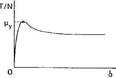
applications) showing shear strength is practically unaffected for a displacement up to 1.5% of the height of the sand specimen. Beyond 1.5% an increase in surface roughness begins to control the coefficient of friction ( s / v), typically monotonically increasing
for tests in dry sand.
Yoshimi initially quantifies surface roughness Rmaxas the maximum difference in the profile (i.e., maximum elevation change) along the continuum material surface.
1
n
max i
i
R
h
(2.1)where hi values are averaged asperity heights for sections along the surface profile of
7 2.5mm, however this value is later revised by Kishida and Uesugi (1987) to 50% of the mean diameter of sand (i.e., D50). This normalized roughness ratio provides more
consistent quantification for a steel surface roughness.
Additional results show that relative density variations from 40% to 90% have little effect on the coefficient of interface friction in dry sand for surface materials: steel, wood, and concrete. This is reasonable because relative density will often govern shear strength of the soil in the sand mass, but in the case of sand-steel interface strength, the influence of relative density at grain-scale contacts is minimal. The type of sand used in interface tests (selected by void ratio, size distribution, water content, and grain shape) shows some change in coefficient of interface friction with respect to angularity of the grains, however it was discovered by Uesugi and Kishida (1986a) in subsequent interface shear tests that the weak influence of grain type may be due to error in the sample preparation, whereby grains did not fully occupying spaces in the rough surface. They argue that if sand is properly pulviated into the rough surface, then grain type has a significant influence over the coefficient of interface friction. Occupation of sand grains in the surface profile valley is aided by a polysize grain size distribution, since smaller particles are likely to fill the gaps. Experiments performed by Abou-Chakra and Tuzun (1999a) using direct shear apparatus highlight the effect of certain heterogeneous particle mixtures of distinct size and roughness on coefficient of interface friction.
particle-8 continuum interface friction angle. This leads to an important feature found for the upper bound with regard to interface shear strength: as increasing surface roughness causes the shear strength to approach an asymptotic limit, it will theoretically reach a friction angle approximately equal to the angle of internal friction in the soil mass. Additionally Yajima et al. (1984) argues that beyond a critical roughness the failure will remain in the bulk soil. This is supported by Yoshimi in tests for rough steel (Rmax = 510μm) where the internal soil friction angle is found to be only a few degrees less than the contact friction angle of the steel-sand interface.
To give some basis for real physical roughness values found in the field Yoshimi and Kishida (1982) reference surface roughness for construction materials at 105kPa normal stress: 10μm to 20μm for steel, 25μm to 90μm for wood, and 50μm to 130μm for concrete. A ring torsion test performed on common rounded sand (i.e., Toyoura sand) measured coefficients of interface friction invariant to normal stresses ranging from 51kPa to 158kPa. Results showed “stick-slip” features evident at Rmax < 5μm pronounced
dilation at Rmax > 220μm. Radiographical observations show slip at the sand-metal interface on the order of 0.1mm to 4.0mm for the majority of test results. A distinct decrease in slope of peak friction angle above 20μm roughness supposes the possible transition of failure mechanism to the sand mass, although this is not mentioned in the study. Importantly, it is noted that the coefficient of friction ( s/ v) is independent of
9 Hence for interface shear tests the normal stress is not necessary to investigate the effect of surface roughness on shear failure mechanism.
Interface shear tests performed by Uesugi and Kishida (1986b) using a simple shear apparatus showed primary factors controlling the coefficient of interface friction (μ = ) are the grain size (i.e., D50) and sand type (i.e., grain roundness). Results are given from two tests: a simple shear apparatus composed of a stack of aluminum frames which allow for shear deformation in the sand mass, and rigid shear box resisting deformation in the sand sample. The total displacement is defined as position change between the bottom plate and the top plate. The interface metal surface is roughened by various machining methods. The surface is cut normal to the direction of sample deformation. A 98kPa normal load is applied to the top of the sample and deformation is measured until shear failure occurs.
Preliminary tests (Uesugi and Kishida 1986a) are performed for the Drrange from 84% to 93%, sub-rounded grain type Toyoura sand, and steel with Rmax ranging from 3.5μm to 19μm. Further tests at more precise roughness gage length are found to match well with Yoshimi and Kishida (1981) for coefficient of friction μ versus roughness data. Additionally a gage length of 0.2mm (significantly smaller than gage length used by Yoshimi) is found to be more closely correlated with Rmax.
10 two sand types, two steel roughness values (approximately 3μm to 20μm), two test types (again simple shear and shear box), and four D50 sizes (ranging 0.16mm to 1.82mm) to
evaluate interface shear test using basic parametric analysis. Results from the experimental design method show D50 had a significant impact on the coefficient of interface friction while the uniformity coefficient, normal stress, whereas the type of test (i.e., direct shear or simple shear) had little impact on the coefficient of friction. Normal stress is shown to influence the sliding displacement during testing but under a certain threshold it is negligible. Uesugi argues roughness Rmax over a given gage length is better correlated with coefficient of interface friction when normalized by D50 as
50 max n
R R
D
(2.2)
where Rmax is defined in Equation 2.1 and D50 is the particle diameter at 50% finer of the
grain size distribution (i.e., cumulative distribution) plot. The critical roughness at which failure mechanism transitions from surface interface to internal soil strength, occurs atRn
of approximately 0.075 (unitless). Uesugi goes on to formulate a quantitative prediction of the coefficient of interface friction based on the normalized roughness and the modified roundness of sand particles.
1
n A B R R
(2.3)
11 microscopic interface, which are correlated to the sand type, steel type, and surface conditions (i.e., dry, wet, lubricated, etc). Theoretically, this adhesion would cause some friction to exist even if the metal surface is infinitely smooth. Uesugi concludes that back-calculated values A0.07 and B0.9 used to estimate coefficient of friction showed good agreement using simple shear and shear box apparatus.
DeJong et al. (2002) argues quantification of interface roughness by Uesugi and Kishida (1986b) is not detailed enough to properly characterize local peaks and valleys in the surface profile. Assuming particle diameter is larger than the width across the surface profile valley, Dejong argues an idealized particle path exaggerates peaks and suppresses valleys in the surface profile. The particle path is similar to a low-pass filter, minimizing the valleys in the surface and smoothing sharp edges in peaks. Gaussian and sharp cutoff filters are employed to compare to the path of particle centroid along the profile geometry. Note that Gaussian and sharp filters are symmetric with respect to peaks and valleys in the surface profile, so the unique effects of particles traversing the surface are lost in both cases.
DeJong plots several measures of surface roughness, including Uesugi‟s Rmax as
well as ASME Standard B.461 average roughness Ra and average slope aas
0 1 L a
R Z x dx
L
(2.4)0 1 L a
dZ dx
L dx
12 for sample length Land absolute value height Z of material above a reference mean elevation axis. Roughness values are given for a theoretical surface using these and several other parameters for particle diameter up to 20mm. For a theoretical surface profile with one valley and one peak, both Raand a are shown to diminish the effect of
the valley for the calculation of surface roughness with increasing particle size. This highlights the effect of valleys versus peaks in the surface profile geometry, which is not considered in Uesugi‟s commonly used measure of surface roughness.
In addition to theoretical results, real physical experiments are performed by Dejong on HDPE geomembrane, tooled steel, and rough finished concrete for a range of particle diameter up to 5mm. HDPE geomembrane and tooled steel show a more dramatic effect in the difference of surface roughness with increasing particle size for both Ra and ∆a, whereas the rough finished concrete show similar trends in surface
roughness irrespective of measurement type. The valley versus peak effect is also more dramatic in materials with irregular surfaces, as shown in trends of particle path compared to Gaussian and sharp cutoff filters of the surface profile. In summary, a more accurate measure of surface roughness is found to be the particle path along the surface profile (i.e., centroid trace method) since it captures local feature, although it is still not clear whether a single best surface roughness parameter exists.
13 profilometer (2μm diameter ball tip), Brinell harness test (with results presented for a 19.0mm sphere indented into continuum material at 250 kgf), and interface shear for two sand types: Ottawa 20-30 and Valdosta blasting sand. A DEM interface friction simulation considers 300 3-grain clusters under 100kPa normal stress. The model is sheared at constant velocity 1.0mm/sec for 10.0mm. Hardness is modeled by changing the surface friction coefficient. Specifically, the softer surface is modeled with higher coefficient of friction which is intended to represent the plowing friction plastic mechanism. Note that DEM is quite useful in revealing individual grain displacements and rotations. Individual grain displacements and rotations are tracked in physical experiment by Uesugi et al. (1988) on a rough surface interface. Results of profilometer tests show Ra lower bound 0.336μm for hardened steel to 115.97μm for rough finished
concrete. Overall it is shown that the normal load, particle angularity, and D50 all influence interface shear strength.
2.2.2 Interface Shear Test Comparisons and Test Simulations
14 infinite displacement range). Simple shear tests tends to exhibit non-uniform error in stress distributions, but are more informative in terms of unique displacement measurements at various elevations than displacements measured by direct shear and ring torsion. Conceptually the simple shear test can be conceived as a modified version of the direct shear test, whereby side walls are discretized so displacement may be measured along many elevation profiles in the soil. For instance, shearing in the bulk sand mass above the sand-steel interface may be correctly measured in the test, as well as displacement occurring solely in the bulk sand mass. The simple shear apparatus accomplishes this by slicing the container into a stack of aluminum plates, each with identical cut-outs containing the sand mass. The bottom plate below the shearing surface is allowed to slide on low friction Teflon plates. Kishida notes that a correction factor is needed to account for the friction generated by the Teflon plates underneath the shearing apparatus. As the test begins, tangential load is gradually increased on the bottom plate until constant sliding is observed at 1mm/sec. Again note displacement may be correctly accounted for along the sand-steel interface and the sand mass, which is not possible in direct shear test.
15 without a great deal of experience and training. Advantages of the simple shear apparatus are also highlighted by Uesugi et al. (1988) to explore detailed microfeatures involved in slip at the sand-steel interface and the shear failure in the bulk sand mass such as emergent behavior caused particle displacements and rotations using X-ray photography. Horizontal translation dominates at low surface roughness corresponding to slip at sand-steel interface, while shear zone is distinctly located in sand mass for the case of rough interface corresponding to inclined sliding and rotating grain movements.
Kishida returns to the problem of quantification of surface roughness Rmax as described previously by Yoshimi and Kishida (1981) defined as the maximum difference in elevation over a certain gage length L (i.e., sampling length), a value of 2.5mm for dry sand. The challenge to determine Rmax lies in the definition of L and orientation of
16 some degree the effect of grain properties such as angularity and qualitative estimations of roughness, but unfortunately distinct binary mixtures are not addressed. This leaves many questions regarding distinct binary mixture effect on the interface strength of sample. The reader is referred to Abou-Chakra and Tuzun (1999b) for a description of qualitative trends given rough or smooth fines in binary mixtures used in direct shear tests.
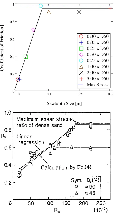
Jensen et al. (1999) addresses the common excessive rotation problem found using DEM by grouping individual disks in to cluster groups. Clusters allow for high granular strength and interlocking behavior characteristic of real physical sand. Each cluster essentially acts as an irregularly shaped particle with additional mass and inertia equal to the sum of constituent particle disks. Clusters may evaluated using Interface Shear Test for a range of surface roughness. Surface roughness is used as previously described by other investigators, where Rmax is essentially defined as the maximum
elevation change in a gage length, averaged over all gage lengths. Jensen defined the inter-particle and particle-wall coefficient of friction to be 0.4 and normal and shear contact stiffness 7.5 x 10⁸ force units per unit length (instead of SI units). Interface shear test cases include 1000 single particle and 3000 3 grain clusters at sawtooth period four times grain diameter4 , 2 , 0.5D D D, with normal stresses ntested range from 5.0 x
17 form in the granular mass and not along the surface. Periodic boundaries are also imposed. Results show as expected shear stress increase with surface roughness and confining stress.
18 Frost et al. (2002) performed interface shear test ASTM D3080 at displacement rate 1.0mm/min for a total of 80mm for normal loads ranging from 50 to 300kPa for Ottawa 20-30 and Valdosta blasting sand where D50 is within 0.1mm but the blasting sand is significantly more angular. For relatively smooth materials like hardened steel, the friction angles where significantly lower than the internal friction angle of the sand, but for rough finished concrete the peak and residual interface friction angles where almost nearly the same as the internal friction angle of the sand. A three-dimensional plot of coefficient of friction with surface roughness and hardness show roughness dominates, while hardness adds friction to achieve upper bound earlier. At low surface roughness, upper bound changes drastically. Again, results agree that the upper bound eventually meets the internal friction angle of the sand regardless of hardness.
19 the corners and side walls since particle movement is increasingly unaffected by surface roughness approaching the boundary. Particle translations from simulation data are plotted and match well with laboratory data (Westgate and DeJong 2006), whereby Ra
and ∆a, as described previously, are employed to compare surface roughness from
simulation to that measured separately by experiment.
Wang goes on to measure the local strain state at several points in the stress-displacement plot including pre-peak, peak, and critical state. Shear bands form in an area concentrated in a mound directly above the rough surface up to roughly 8 to10 times
20 Wang et al. (2007b) goes on to provide a quantitative correlation for shear strength criterion based on surface roughness. The method computes eigenvectors in the principle directions from the contact forces at grain-interface (Bathurst & Rothenburg 1989 ; Santamarina 2001) surface for two sampled regions: the first region consists of contacts directly along the rough surface, and another rectangular region 14mm above the surface. According to Rothenburg the sum of eigenvalues approximates the mobilized internal friction angle:
1
2
mobilized c n t
sin a a a (2.6)
1 31 3 mobilized
sin
(2.7)
where 1 and 3 are the principle stresses, ac is the anisotropy in contact orientation, an
is the anisotropy in normal force, and at is the anisotropy in shear force. These values are
a function of particle displacements, and may be extracted from the Fourier series fit to the distribution contacts or force components at selected grain pairings as
1
1 2
2 c a
E a cos
(2.8)
0 1 n 2
n
N N a cos (2.9)
0 t 2
t
T N a sin (2.10)
21 of interparticle force chain for sawtooth and geomembrane surfaces dominate in the direction of n reaction to the surface profile.
Wang goes on to define the principle direction a as the interface contact normal
determined from the particle centroid path along a sawtooth surface profile as described previously by DeJong. Then parameter a is correlated to t and n using DEM,
subsequently relating principle directions a to r. This provides a prediction of r
given a from only the surface profile geometry. The resultant r is important since it
approximates the friction angle at interface from the Mohr-Coulomb criterion.
Interface shear is a fundamental phenomenon controlling granular material properties and interface mechanics. Behavior at interface is well studied but limited applications to soil-structure interaction models have been made, particularly using discrete numerical approach. DEM may be used to capture interface shear behavior such as surface roughness effects on shear failure mechanism. Directivity at particle-continuum contacts is a major factor in the failure mechanism as observed numerically using strength tests. Direct implications to the effect of soil failure in soil-structure interaction models naturally follow.
2.3 Shallow Foundations
2.3.1 Bearing Capacity
22 of the bearing capacity equation from limit equilibrium for cohesionless soils. Early work by Rankine provides a basis for bearing and settlement theory in the 20th century (e.g., Rankine passive soil zone is implemented by Terzaghi). Subsequently Prandtl (1920) as referenced in Bowles (1996) developed a theory of plastic equilibrium analyzing a punching wedge of softer material (i.e., weightless soil) under a rigid base. The wedge implies a failure surface and slip mechanism and is essentially solved as a free-body force diagram, achieved specifically by the method of characteristics (i.e., slip-line method). Slip surface geometry are later adopted by Terzaghi, Prandtl to obtain Nc
and Nqbearing coefficients.
Terzaghi (1943) defined the widely used form of the bearing capacity revised from Prandtl theory for a continuous foundation in two dimensions as
0 5 ult
ult c z q Q
q cN N . BN
A (2.11)
where c is cohesion, z is the vertical effective stress, is the soil self-weight, B is the
foundation width, and Nc, Nq, N are the cohesion, overburden, and soil self-weight
bearing capacity factors respectively. The final form of the classic equation considers the bearing as a function of three terms: cohesion, foundation loading, and soil self weight. The self weight factor N is still controversial and many more accurate definitions have
23 Assumptions made for the bearing capacity equation include: BD (where D is depth of embedment), zero base shear (i.e., infinite roughness), homogeneous soil extending infinitely below foundation (i.e., , c, and γ constant with depth), applicability of simplified Coulomb envelope tan( ) , governing general shear failure mode, rigid foundation, and requirement that any soil above foundation acts only as surcharge. Terzaghi defines three zones which may be physically observed as soil fails and foundation base contact stress approaches ultimate bearing capacity. Failure zones include an elastic wedge directly beneath the base, Prandtl radial shear zone (log spiral slip surface or special case circular slip surface for clean coarse-grained soils), and Rankine passive linear shear zone. The failure surface in the linear zone is extended up to ground level by Meyerhof (1951) as referenced by Bowles (1996) for cases when foundation depth is greater than zero. Note that Rankine passive linear zone is oriented at 45 2 and log spiral surface depends on B/z, where is the soil unit weight, B is the foundation width, and z is stress applied in the vertical direction.
24 Possible failure modes which are defined by Vesic (1973) for Chattahoochee sand under a circular foundation. These included general, local, and punching failure. Factors such as foundation depth, void ratio, and grain size, and relative density control the type of failure mode. General failure is expected for shallow foundations. General failure represents the most brittle dense incompressible material while punching failure represents the most plastic loose compressible material. General failure also produces ground heave, while deformation is restricted to a region below the foundation in local and punching failure. From general to punching failure the load displacement curve will reveal less defined ultimate bearing capacity (i.e., there exists no clear maximum load value).
2.3.2 Improvements to the Bearing Capacity Equation
Although Terzaghi assumed concentric loading this is not typically the case in the field. Distribution of contact forces along the foundation base measured in the field are affected by load eccentricity, local soil property variation, and variation in roughness along the base surface. Many of the analytical revisions consider eccentric loadings and inclination along embankments, such as ground inclination factors are provided by many of the authors listed in Section 2.3.2.
Although Nc and Nqbearing coefficients are well accepted, the soil self weight
term N (Caquot 1953) as referenced in Budhu (2008) is problematic. Kumbhojkar
25 after further review it is found to offer little improvement to Terzaghi‟s original values (Bowles 1996). The reader is referred to Section 2.3.7 which discusses attempts to determine the most accurate values of N via numerical methods (e.g., Finite Element
Method) by investigators Ukritchon et al. (2003) and Yamamoto et al. (2009).
Adjustments to the friction angle and cohesion are also common, since peak friction is extremely important for an accurate solution of the bearing capacity equation. Bolton (1986) as referenced by Budhu (2008) gave a more precise account for the changing angle of dilation along the failure surface and provided a correction factor for the peak friction angle. Another error caused by superposition is found in bearing capacity equation by Sloan (1996) as referenced by Salgado (2008) and Michalowski (1997).
Ueno (1998) provides a method for extracting and c from principle stresses and foundation width B. These parameters may then be input into traditional analytical bearing capacity formula. Ueno provides the theoretical framework in terms of mean principle stress σm = (σ1 + σ3)/2. The friction angle and cohesion intercept are determined
by a τm-σm graph (mean shear and normal stress, respectively). This information can also
26 Finally, in-situ bearing capacity correlations have the advantage of being much less expensive than full-scale or even reduced scale footing tests. Early solutions for the bearing pressure predicted from SPT results are provided by Terzaghi and Peck (1967) as referenced by Reese (2006). Meyerhof (1965) as referenced by Budhu (2008) estimated bearing capacity from N1 (corrected for overburden pressure) from SPT test.
2.3.3 Settlement
Settlement is classified as immediate (i.e., elastic), primary (i.e., consolidation), and secondary (i.e., creep), where soil settlement is often derived from the consolidation curve plotted in logarithmic scale which is assumed to by one dimension acting with all strains along the vertical axis. For normally consolidated soils this is given as
0 0 0 1 f primary c z H C log e
(2.12)
where H0 is the height of soil layer, e0 is the initial void ratio, Cc is the slope of
consolidation curve from lab test, and f z 0 is the ratio of final to initial vertical
27 easily drain around the boundary of the compression volume in the field, leading to increased settlement in the field. Also for prediction of a multilayer system, the one-dimensional consolidation equation assumes all layers consolidate based on hydrostatic and surcharge stresses, where top layers are often recommended to be smaller and increase with depth.
Overall the best way to know how soil response will scale is to run a full field test, but this is expensive and impractical, so well correlated factors are most often used, whether applied to results consolidation lab or in-situ estimates. Another shortcoming of the one-dimensional consolidation method is that settlement is not completely influenced by vertical load. Soil above the foundation is shown to decrease settlement by providing increased confinement effect (Gazetas and Stokoe 1991), where a fraction of foundation load is resisted by side wall shear resistance, reducing vertical settlement. Accordingly, extraneous effects such as these must be taken into consideration in the development of analytical and numerical solutions.
Classic analytical methods for prediction of immediate (i.e., primary) settlement of shallow foundations originate from elastic theory where typical parameters include soil modulus of elasticity and Poisson‟s ratio. Generally an elastic analytical solution can take a form similar to that given by Poulos for deep foundations
2
1
B
q I
EL
28 where qis the load, B is the pile width, is the Poisson ratio, E is the elastic modulus for the soil, L is the pile length, and I is an influence factor. The soil elastic modulus may be estimated by a variety of methods: analytical solution by theory of elasticity, unconfined compression test (which gives lower bound values), Triaxial compression test (which gives most likely values), in-situ testing (SPT, CPT, and Pressuremeter), and Plate-Load test in the field (Bowles 1996). Immediate settlement of the corner of rectangular base on surface of elastic half-space, approximating soil, is derived from theory of elasticity (Timoshenko and Goodier 1951) as referenced by Bowles (1996). One limiting assumption for the solution provided by Steinbrenner is that the foundation is perfectly flexible. For the elastic settlement Bowles (1987) recommends weighted average for soil elastic modulus over multiple layers since the modulus is not constant in the real field case. Gazetas et al. (1985) as referenced by Budhu (2008) gave a solution for immediate settlement of foundation of arbitrary shape (as seen from plan view) using elastic theory. The most challenging factor in most elastic methods to determine is the undrained soil modulus Eu (where accuracy of Eu may be determined from undrained Triaxial testing).
29 (1970) as referenced by Budhu (2008), which considers total settlement as the sum of individual strains over the depth of penetration, with other factors considering shape and depth similar to the traditional bearing capacity equation. The Schmertmann estimate hinges on an empirically correlated influence factor attributed to each layer divided by the Young‟s Modulus of each layer. Settlement is computed as a function of cone tip resistance as described by several investigators (Schmertmann 1970 ; Lee and Salgado 2005). Burland and Burbridge (1985) as referenced by Budhu (2008) estimated bearing capacity from Nuncorrected which is a function of foundation width, hydrostatic pressure,
blow count or cone resistance, and grain size from 200 foundation tests in sand and gravel. From this statistical analysis an estimate for settlement is proposed in terms of shape, influence, and correction factor.
2.3.4 Model Testing
30 described by Muhs and Selig. Shallow foundations on sand have high ultimate bearing capacity and it is difficult to induce failure in full-scale load tests. The accuracy of bearing capacity analysis is explored in full-scale experiments by Bishop for fourteen load tests on saturated clays and by Briaud and Gibbons (1994) as referenced by Bowles (1996) for five static load tests on spread footings in silty fine sand. Briaud found silty fine sand did not reach failure for full-scale load tests, even up to 150mm displacement. Hence in practice the design criterion is most often governed by settlement instead of bearing. Settlement tests are also performed on simple plate loads by Terzaghi and Peck (1967) and D‟Appolonia et al. (1968) as referenced by Bowles (1996), but these are
found to underestimate actual settlement by factor of two.
31 Akbas and Kulhawy (2009a) provide predictive curve fitting method for shallow foundations from a large database of full scale load tests performed on cohesionless soil. Methods in consideration such as 10%B, L1-L2, and tangent intersect method, are all used to quantify load test results, after which and statistical deviation and variance are measured. Methods with highest correlations are ratios of Q%10B/QL2 and QL2/QTI. Since
2 L
Q has highest correlation with other methods, the hyperbolic fit proposed by Akbas
features the mean stress normalized by QL2 as
2 L Q
B a B b
Q (2.14)
where Q is the load, is settlement at the base, and B is the foundation width. Using parameters mean values of a and b curve fit to the large database of experimental results the hyperbolic equation predicts expected load-settlement behavior. Akbas and Kulhawy (2009a) also go on to link the soil modulus to the initial linear elastic region of the load-settlement curve in a modified form normalized by the atmospheric pressure. The bearing capacity can also be informed by the testing database. An analytical equation based predominantly on the Vesic (1973) formulation is found to correlate well with QL2
(such that r2 = 0.99) based on the ratio QVesic QL2 when B > 1m but becomes less
32 and is shown to match reasonable well (r2 = 0.74) for a subgroup containing the best data available from the test database.
Of last note with regard to foundation settlement, it is found that with respect to model scale problems, several investigators (Briaud and Gibbens 1999 ; Pardo and Bobet 2007 ; Akbas and Kulhawy 2009a) agree that normalized settlement B tends to help minimize foundation size effects on settlement-stress response, collapsing data of various foundation width to a narrow range.
2.3.5 Induced Stress
Boussinesq produced a classic solution for induced stresses in elastic material due to applied forces enhanced with influence factor by Newmark (1935) and Westergaard (1938) as referenced by Bowles (1996). Westergaard gives estimate of stress in soil from surface load in which solution addresses the same problem as Boussinesq yet derived from slightly different assumptions. The methods described so far for solution of induced stress field are difficult to solve analytically, so a simple approximated method is given by Poulos and Davis (1974) for circular foundations. More sophisticated solutions are useful for description of the stress field, and may be developed from stress-strain relationship as the discrete load function where solution is aided by Fourier Transform.
2.3.6 Numerical Methods
33 and internal friction angle. Also, numerical solutions are flexible for a multitude of foundation geometries and loadings. Advantages include the ability to monitor mechanical behavior of individual soil elements across spatial extents. FEM and FDM solutions are available in commercial software packages such as FLAC, PLAXIS, and ABAQUS.
Loukidis and Salgado (2009) determined the bearing capacity factors, shape factors, and dilation angle using finite element simulations and analytical methods (i.e., limit analysis and method of characteristics). Results showed FEM bearing capacity value within 2.5% of analytical solutions. Griffiths and Fenton (2009) predict elastic settlement of a strip footing on variable soil. They investigated the limit state design (i.e., settlement, bearing capacity, serviceability) reliability based uncertainty. Results are also compared by statistical analysis. Specifically stochastic finite element methods and random finite element methods are compared. Low stiffness values assigned in the random field dominated mean settlement. Stochastic FEM underestimated the probability of failure when compared with the random field FEM approach.
An FEM study on bearing capacity of the upper and lower bounds for the controversial bearing capacity equation coefficient N is made by Ukritchon et al.
34 solution decreases significantly at a friction angle above 30°. Overall results for N from Ukritchon‟s FEM model agree well with Hansen and Christensen (1969) and Booker (1969) for a wide range of friction angles (from 15° to 45°). Ukritchon‟s results disagreed with Terzaghi (1943) and corresponding description by Vesic (1973) which seem to overestimate N by approximately a half order of magnitude on rough footing.
Yamamoto et al. (2009) uses a 13 input MIT-S1 model (of which only 3 parameters are deemed to have much influence over results) to determine the foundation width effects on the value ofN . The asymptotic approach of N to an upper bound is
consistent for siliceous sands, more slowly for calcareous sands. For both soil types Yamamoto‟s results support the significance of the foundation size effect on the bearing capacity factor.
35 2.4 Deep Foundation
2.4.1 Pile Installation
36 2.4.2 Load-Deformation
Compared to typical shallow foundations the ultimate load in deep-foundations is often difficult to determine. This is partly due to additional load carried by side friction which lessens the pronounce peak failure evident in shallow foundation cases. Side friction is often assumed to mobilize within 5mm to 10mm approaching 10%B (Coduto 2001). Curve fitting models are quite popular for quantifying load-deformation q-δ test data, for deep foundations, formulations based on q-δ are provided by several
investigators (Van der Veen 1953 ; Chin 1970 ; Davisson 1975 ; Fellenius 1999) as referenced by Salgado (2008). Of these studies, Davisson‟s solution is often too conservative. Davisson predicts the failure load as a function of three terms: 0.15in mobilization between side wall and soil, B/120 settlement due to toe failure, and elastic compression of the pile.
1 0 15
120 ult
PL
. in B
EA
(2.15)
where E is elastic modulus of the pile material, P is the load,L is pile length, A is pile cross sectional area, andB is the pile width. Davisson‟s equation graphically linear with slope L/AE and settlement axis intercept 0.15in + 1/120B.
2.4.3 Bearing Capacity
37 capacity equation is used to estimate toe resistance as a function of soil self-weight controlled by the lateral earth pressure coefficient. Hence, the failure mechanism, if controlled at least partially along the side, is likely to occur at a greater depth along the pile wall instead of near the surface. The failure process, specifically the emergence of various failure lines and plastic zones in the region near the pile toe begins with punching failure wedge and evolves to full general shear failure with log spirals slip surfaces if the pile is displaced further, although failure will often reach only punching or local modes. Overall, bearing capacity is controlled by: internal angle of friction, cohesion, soil unit weight, and relative density.
Pile dimensions and soil properties control whether the side (i.e., friction pile) or toe (i.e., end-bearing pile) failure mechanism dominates. Typically dry course soil experiences greater side resistance than toe resistance due to the large surface area of the side of pile which generates significant friction. Ultimate bearing may be computed by the general formulation
total side toe
Q f A q A (2.16)
where q is similar to the formulation of Terzaghi‟s bearing capacity and f is a measure
of the effective overburden stress and lateral earth stress K0z, and Aside, Atoe are the
pile side and toe areas respectively. Allowable load capacity is the factored ultimate load. Toe capacity may be predicted by the general bearing equation as
2 toe
zD q P
BN N