Fine Mapping Causal Variants with an Approximate Bayesian Method Using Marginal Test Statistics

(1)

HIGHLIGHTED ARTICLE

GENETICS | INVESTIGATION

Fine Mapping Causal Variants with an Approximate

Bayesian Method Using Marginal Test Statistics

Wenan Chen,* Beth R. Larrabee,* Inna G. Ovsyannikova,†_{Richard B. Kennedy,}†_{Iana H. Haralambieva,}† Gregory A. Poland,†_{and Daniel J. Schaid*},1 *Division of Biostatistics and†Mayo Clinic Vaccine Research Group, Mayo Clinic, Rochester, Minnesota 55905

ABSTRACTTwo recently developedfine-mapping methods, CAVIAR and PAINTOR, demonstrate better performance over otherfi ne-mapping methods. They also have the advantage of using only the marginal test statistics and the correlation among SNPs. Both methods leverage the fact that the marginal test statistics asymptotically follow a multivariate normal distribution and are likelihood based. However, their relationship with Bayesianfine mapping, such as BIMBAM, is not clear. In this study, wefirst show that CAVIAR and BIMBAM are actually approximately equivalent to each other. This leads to afine-mapping method using marginal test statistics in the Bayesian framework, which we call CAVIAR Bayes factor (CAVIARBF). Another advantage of the Bayesian framework is that it can answer both association and fine-mapping questions. We also used simulations to compare CAVIARBF with other methods under different numbers of causal variants. The results showed that both CAVIARBF and BIMBAM have better performance than PAINTOR and other methods. Compared to BIMBAM, CAVIARBF has the advantage of using only marginal test statistics and takes about quarter to

one-ﬁfth of the running time. We applied different methods on two independent cohorts of the same phenotype. Results showed that CAVIARBF, BIMBAM, and PAINTOR selected the same top 3 SNPs; however, CAVIARBF and BIMBAM had better consistency in selecting the top 10 ranked SNPs between the two cohorts. Software is available athttps://bitbucket.org/Wenan/caviarbf.

KEYWORDSBayesianﬁne mapping; marginal test statistics; causal variants

U

NTIL recently, there have been .2000 genome-wide association studies (GWAS) published with different traits or disease status (Hindorffet al.2014). Most of them reported only regions of association, represented by SNPs with the lowestP-values in each region. Only a few provide further information of likely underlying causal variants. A noted exception is reﬁnement based on Bayesian methods (Malleret al.2012). Fine mapping the causal variants from the veriﬁed association regions is an important step toward understanding the complex biological mechanisms linking the genetic code to various traits or phenotypes.

Fine-mapping methods can be roughly divided into two groups. Theﬁrst group was developed before the availability of high-density genotype data. These ﬁne-mapping methods assume the causal variants are not genotyped in the data and

aim to identify a region as close as possible to the causal variants (Morriset al.2002; Durrantet al.2004; Liang and Chiu 2005; Zollner and Pritchard 2005; Minichiello and Durbin 2006; Waldron et al. 2006). Because the causal variants are not observed in the data, these methods usually rely on various strong assumptions to model the relationship of the causal and the observed variants. Examples include models based on the coalescent theory (Morris et al. 2002; Zollner and Pritchard 2005; Minichiello and Durbin 2006) or statistical assumptions about the patterns of linkage disequilibrium (LD) (Liang and Chiu 2005). There are at least two limitations of these methods. First, the result is usually a region with a conﬁdence value rather than candidate causal variants. Second, the result may be unreliable if the model assumptions are too strict and deviate far away from the real data, or the inferred region may be too wide to be useful if the model assumptions are too general.

The second group ofﬁne-mapping methods assumes that the causal variants are among those measured. As the se-quencing technology advances and with the availability of the HapMap Project (Altshuler et al. 2010) and the 1000 Genomes Project (Abecasiset al.2012), it is feasible to obtain the sequence data of the association regions or impute almost

Manuscript received March 6, 2015; accepted for publication May 4, 2015; published Early Online May 6, 2015.

Supporting information is available online at www.genetics.org/lookup/suppl/

doi:10.1534/genetics.115.176107/-/DC1.

1_{Corresponding author: Division of Biostatistics, Harwick 7, Mayo Clinic, 200 First St.}

(2)

all common variants with high quality. Now it is plausible to assume the causal variants exist in the data, either mea-sured or imputed. How to best prioritize the candidate causal SNPs for follow-up functional studies becomes the aim ofﬁne mapping (Fayeet al.2013). One simple way to prioritize variants is based onP-values. However, there are at least two limitations of this method. First, P-values do not give a comparable measure of the likelihood that a var-iant is causal across loci or across studies (Stephens and Balding 2009). Second, a noncausal variant could have the lowestP-value due to LD with a causal SNP and statistical

ﬂuctuation. This may also happen when a noncausal vari-ant is in LD with multiple causal SNPs.

There have been several methods developed to address the above problems. For example, in Malleret al.(2012), a Bayesian method was developed to refine the association signal for 14 loci. This method circumvents the first limitation of using P-values by using the posterior inclusion probability (PIP). How-ever, it assumes only a single causal variant for each locus. Recently, two fine-mapping methods, CAVIAR (Hormozdiari et al. 2014) and PAINTOR (Kichaev et al. 2014), were pro-posed, which lift the restriction of a single causal variant in a locus and show much better performance than otherfi ne-mapping methods. Another advantage is that only the mar-ginal test statistics and the correlation coefficients among SNPs are required, instead of the original genotype data, which makes it easier to share data among different groups. When only marginal test statistics are available, which is not uncommon, the correlation among SNPs in a study can be approximately computed from an appropriate reference pop-ulation panel,e.g., from the 1000 Genomes Project. We noted that BIMBAM (Servin and Stephens 2007; Guan and Stephens 2008), a Bayesian method, can be used forfine mapping mul-tiple causal variants by setting the maximal number of causal variants allowed in the model. Both CAVIAR and PAINTOR use the marginal test statistics directly and are likelihood based. The relationship with other Bayesian methods, such as BIMBAM, which takes the original genotype data as input, is not clear. In this study, we derive and explain the relation-ship between CAVIAR/PAINTOR and BIMBAM, which leads to a unified Bayesian framework for bothfine mapping and as-sociation testing using marginal test statistics. We call our proposed method CAVIAR Bayes factor (CAVIARBF). We also compared the performance of differentfine-mapping methods in simulations with multiple causal variants.

Compared to CAVIAR, PAINTOR has an additional op-tion to include extra funcop-tional annotaop-tions about the variants. Even though it is important to include the anno-tations when they are available, we focus on the scenario where no annotation is available and discuss functional annotations in the Discussion. There are other Bayesian-based methods in ﬁne mapping, such as those in Wilson et al.(2010) and Guan and Stephens (2011). These methods are based on sampling techniques, such as the Markov chain Monte Carlo (MCMC) algorithm. Because MCMC methods can require more computation time than BIMBAM or CAVIARBF,

where the Bayes factors are calculated analytically and exhaustively enumerated, MCMC methods have compu-tational limitations. We further discuss these issues in the Discussion.

Materials and Methods

Approximate equivalence between BIMBAM and CAVIAR

In this section we derive the equivalence between BIMBAM using a D2prior and CAVIAR. SupposeXis ann3mSNP

matrix. It is coded additively as 0, 1, and 2 for the number of a speciﬁed allele for each SNP, wherenis the number of individuals and m is the number of putative causal SNPs. First, we scaleXso that each column ofXhas mean 0 and variance 1;i.e.,ð1=nÞPn_i_¼₁Xij¼0;ð1=nÞ

Pn i¼1X

2

ij ¼1; j¼1;2;. . .;n:Xijis the element of rowiand columnjinX.

The quantitative phenotype yis a n3 1 vector. We also centeryso that we can use the linear model without the intercept as

y¼Xbþe; (1)

where b is the effect size and eNð0;ð1=tÞIn). Here In

denotes then3nidentity matrix.

Bayes factor from BIMBAM using the D2prior givent:The D2 prior from Servin and Stephens (2007; Guan and

Stephens 2008) assumes thatbhas a prior normal distribu-tion N(0,vð1=tÞ), wherevis a diagonal matrix andbande are independent. Assume all SNPs have the same variance s2

að1=tÞ;i.e.,v¼s2aIm:Then we have

Eðyjt;XÞ ¼EðEðyjt;X;bÞÞ ¼EðXbÞ ¼0;

Varðyjt;XÞ ¼EðVarðyjt;X;bÞÞ þVarðEðyjt;X;bÞÞ

¼E

1 tIn

þVarðXbÞ

¼1_tðInþXvXTÞ:

Note that XT _{means the transpose of}_X_:_Since _y_{is a linear}

transformation of the multivariate normal random vector

ðb;eÞT

;yhas a normal distribution

yt;X N

0;1_tInþXvXT

: (2)

The likelihood of model (1) is Pðyjt;XÞ ¼

ð2pÞ2ðn=2ÞjDj2ð1=2Þexpð2ð1=2ÞyTD21yÞ; where D¼

ð1=tÞðInþXvXTÞ: The null model is that b¼0;i.e., v¼0 Im ors2a¼0:Therefore the likelihood of the null model is P0ðyjt;XÞ ¼ ð2pÞ2ðn=2ÞjD0j2ð1=2Þexpð2ð1=2ÞyT_D21

0 yÞ; where

(3)

BF1¼ ð

2pÞ2ðn=2ÞjDj2ð1=2Þexp2ð1=2ÞyTD21y

ð2pÞ2ðn=2ÞjD0j2ð1=2Þexp2ð1=2ÞyT_D21 0 y

¼InþXvXT2ð1=2Þexpð21

2y T_I

nþXvXT

21 ytþ1

2y T_yt_Þ:

From the Woodbury matrix identity (Harville 2008),

ðInþXvXTÞ21¼In2Xðv21þXTXÞ21XT;resulting in

BF1¼InþXvXT2ð 1=2Þ

exp

1 2y

T_X_v21_þ_XT_X21_XT_yt

:

Bayes factor from CAVIAR givent:SupposeXhas full col-umn rank. From result (2), we have

1

ffiffiffi

n

p XTyt;X N 0;1 t

XT_X n þ

XT_XvXT_X n

!! :

Let Sx¼XTX=n; which is the correlation matrix among

SNPs inX. We can write 1

ffiffiffi

n

p XTyt;X N 0;1_tðSxþSxðnvÞSxÞ

! ⇔ 1ffiffiffi

n

p XTy

ð1=tÞ1=2

Nð0;SxþSxðnvÞSxÞ:

Let u¼nv and z¼ ð1=pffiffiffinÞðXT_y_=ð₁₌_t_Þ1=2_Þ_;

then zNð0;SxþSxuSxÞ: If the variance 1=t is replaced by

the maximum-likelihood estimate from the linear model (1) when keeping one SNP in the model at a time, the resulting vector ^z¼ ðz1;z2;. . .;zmÞT consists of exactly the marginal

test statistics for each SNP used in CAVIAR (Hormozdiari et al.2014). The likelihood ofzis

Pðzjt;XÞ ¼ ð2pÞ2ðn=2ÞjSxþSxuSxj2ð1=2Þ 3exp

21

2z T_ðS

xþSxuSxÞ21z

:

For the null model,u= 0, the likelihood ofzis

P0ðzjt;XÞ ¼ ð2pÞ2ðn=2ÞjSxj2ð1=2Þexp

21

2z T_ðS

xÞ21z :

Then the Bayes factor based on zis

BF2¼

_SxþSxuSx2ð1=2Þexpð2ð1=2ÞzTðSxþSxuSxÞ21zÞ

_S_x2ð1=2Þ

expð2ð1=2ÞzT_ðS xÞ21zÞ

:

BecauseXhas full column rankm,Sxalso has rankmand is

nonsingular. Therefore,

_S_x_þ_S_xuSx¼SxðImþuSxÞ¼SxImþuSx

¼SxImþvXTX:

From Sylvester’s determinant theorem (Harville 2008),

ImþvXTX¼InþXvXT:Therefore,

_S_x_þ_S_xuSx¼SxInþXvXT:

From Woodbury matrix identity, ðSxþSxuSxÞ21¼

S21

x 2ðu21þSxÞ21;resulting in the Bayes factor

BF2¼InþXvXT2ð 1=2Þ

exp 1 2z

T_u21_þ_S x

21 z

! :

By plugging in the deﬁnition ofzandu,

BF2¼InþXvXT 2ð1=2Þ

exp 1 2 1 ny T_X 1 nv

21_þ1 nX

T_X

₂1 XTyt

!

¼InþXvXT 2ð1=2Þ

exp

1 2y

T_X_v21_þ_XT_X21_XT_yt

¼BF1:

Therefore, givent, BIMBAM (usingD2prior) and CAVIAR

have the same Bayes factor. In practice, t is unknown. BIMBAM uses a noninformative prior for t and integrates it out. On the other hand, CAVIAR uses the maximum-likelihood estimate (MLE) of 1=tby putting one SNP at a time in model (1);i.e., only one column ofXis used each time. There are two approximations here. First the MLE is used instead of the true unknown 1=t:Second, different MLEs of 1=t from dif-ferent columns of X are used for each element of z. The second approximation makes the result of CAVIAR farther away from a true Bayes factor. An alternative approximation is to use the MLE of 1=t from model (1) with the full X matrix. However, this loses the ability to directly use marginal test statistics. Forﬁne mapping of a region, because SNPs in a region usually explain only a very small portion of the total variance ofy,e.g.,,5%, the MLEs from different columns ofXmay be all close to the true parameter. In practice, the calculated Bayes factors from CAVIAR and BIMBAM are usually similar to each other, given that the samevis used. In the CAVIAR article (Hormozdiariet al.2014), all SNPs in a region are used in calculating Bayes factors. The varian-ces of the SNPs not in the putative causal model are set to a very small positive value. When this value approaches 0, the result approaches the case where only putative causal SNPs are used as above. Using only putative causal SNPs to com-pute the Bayes factor can also be faster. Another advantage of the above derivation is that even whenXis not full column rank, which is very common for SNPs in high LD, we can still use the following formula to calculate the Bayes factor:

BF2¼ImþnvSx 2ð1=2Þ

exp 1 2z

T_ð_nv_Þ21_þ_S x 21 z ! : (3) For small u¼nv; e.g.,u21_.₁₀23_;_{this avoids the need to}

add a small positive value to the diagonal of Sx; which is

(4)

may be unstable. In this case we still need to add a small positive value to the diagonal of Sx; e.g., 1023: This may

have some shrinkage effect on the Bayes factors compared to that from BIMBAM based on our simulations. Our imple-mentation of CAVIARBF is based on Equation 3.

BIMBAM can naturally incorporate a dominance effect by adding an extra column toXfor each SNP, which is coded as 1 for the heterozygous genotype and 0 for others. The same could be used for CAVIAR to extend it to incorporate a domi-nance effect. In this case, each SNP will have twozstatistics calculated, one for the SNP column of additive effects and the other for the heterozygous indicator. The correlation matrix also needs the correlations with these heterozygous indicators. In the above proof, we assumed that the SNP matrixXis scaled to have variance 1 for each SNP. This is not assumed in the BIMBAM article (Servin and Stephens 2007; Guan and Stephens 2008). In the following we consider the im-pact of scaling. As noted in Guan and Stephens (2011), scaling to variance 1 corresponds to a prior assumption that SNPs with lower minor allele frequency have larger effect size. Speciﬁcally, suppose X~ is the original centered SNP matrix, but not scaled, with the model

y¼Xg~ þe;

where gNð0;wð1=tÞÞ: Then the scaled SNP matrix X¼Xs~ 2ð1=2Þ_;_where_s_{is the diagonal matrix with the variance}

of each SNP on the diagonal. FromXb¼Xs~ 2ð1=2Þ_b_¼_Xg~ _and

bNð0;vð1=tÞÞ;we have the correspondence thatvi¼siwi;

subscript idenotes theith diagonal elements. If we assume a common priorvi¼s2afor all SNPs in the scaled SNP matrix X, thenwi¼s2a=si;which is proportional to the inverse of the

SNP i’s variance in the originalX~:On the other hand, if we assume a common prior wi¼s2a in the original X~; then vi¼sis2a; which has a smaller value if the minor allele

fre-quency is low. Since there is no strong reason to prefer one to the other, in our software we provide the option to set the weightsi for each SNP in the implementation of CAVIARBF.

To get results similar to those of BIMBAM, we just need to set the weightsito the variance of the corresponding SNPs.

PAINTOR (Kichaev et al.2014) is a recently proposed method to prioritize causal variants that can optionally include additional function data. Without function data, PAINTOR is similar to CAVIAR. Both use marginal test statis-tics and SNP correlations and leverage the multivariate nor-mal distribution. However, PAINTOR does not model the uncertainty of the effect size (or noncentrality parameter) as in CAVIAR. Instead, it uses the observed test statistic as the true underlying effect size if the observed test statistic is larger than a threshold. This may result in a decrease in performance when the observed data deviate largely from the true values.

Model space, Bayes factors, and posterior inference

To compute the probabilities of SNPs being causal, we need to consider the set of possible models to evaluate and their related Bayes factors. Suppose the total number of SNPs in

a candidate region isp. Letc¼ ðc1;c2;⋯;cpÞwith each

com-ponent being either 0 or 1, indicating whether the corre-sponding SNP is in a causal model. The total number of possible causal models is 2p_:_{It is usually prohibitive to}

enu-merate all models whenpis relatively large,e.g., forp.20. Similarly as in Hormozdiariet al.(2014), we set a limit on the number of causal variants in the model, denoted byl; e.g., l = 5. This reduces the total number of models to evaluate in the model spaceMtoPli¼0

p i ;where p i

denotes the number of i combinations from p elements. For any causal model Mc in the model spaceM, we can

calculate the posterior probability as

pðMcjDÞ ¼pðMc;DÞ pðDÞ ¼

pðDjMcÞpðMcÞ

P

Mt2MpðDjMtÞpðMtÞ ;

where Ddenotes the data. For example, for BIMBAM,D¼

ðy;XfullÞ;whereXfullrepresents all SNP data. For CAVIAR/

CAVIARBF, D¼ ðzfull;SfullÞ; where now the marginal test statistics and the correlation matrix represent the data. The prior probabilities ofMcandMtarepðMcÞ and pðMtÞ;

respectively. Denote by M0the null model where no SNP

is included; i.e., c¼ ð0; 0;⋯;0Þ: Deﬁne the Bayes factor comparing modelMc with the null model by BFðMc:M0Þ ¼

pðDjMcÞ=pðDjM0Þ: The posterior probability of each model can be calculated as

pðMcjDÞ ¼P BFðMc:M0ÞpðMcÞ Mt2MBFðMt:M0ÞpðMtÞ

: (4)

The posterior probability of the global alternativeMgthat at

least one SNP is causal in the region can be calculated as

pðMgjDÞ ¼

P

Mt2MgBFðMt:M0ÞpðMtÞ P

Mt2MBFðMt:M0ÞpðMtÞ :

We can also use Bayes factors to compare the global alterna-tiveMg with the null modelM0 (Wilsonet al.2010), which

can be calculated as

BFðMg:M0Þ ¼

P

Mt2M_PgBFðMt:M0ÞpðMtÞ

Mt2MgpðMtÞ :

As advocated in Servin and Stephens (2007; Stephens and Balding 2009; Wilson et al. 2010), the Bayesian method provides a natural way to answer both the association ques-tion (Which regions are most likely associated with the phe-notype?) and theﬁne-mapping question (If a region shows evidence of association, which are the potential causal SNPs in the region?). In the following we focus on theﬁne-mapping question.

Marginal PIP

(5)

pðcj¼1jDÞ ¼

X

Mc2M;cj¼1

pMcD:

Here we provide a justiﬁcation of using marginal posterior probability to rank SNPs. Suppose we want to selectkSNPs fromp SNPs, and our objective is to maximize the number of causal SNPs among thesekSNPs. Denote the indexes of the selected k SNPs by Ik: The objective value is then q¼P_j₂_I_kcj:Because eachcjis a random variable, it is

natu-ral to use the expectationEðqjDÞas the objective function. It turns out that EðqjDÞ is the sum of marginal PIPs of the selectedkSNPs as follows:

EðqjDÞ ¼E X j2Ik

cjD

!

¼X

j2Ik

EðcjDÞ ¼

X

j2Ik

pðcj¼1jDÞ:

To maximizeEðqjDÞ;we need only to sort allpSNPs based on their marginal PIPs and choose the topkSNPs. In other words, prioritizing SNPs based on marginal PIPs maximizes the expected number of causal SNPs for afixed number of SNPs selected. There are two implications from this result. First, when selecting SNPs from multiple loci, we need to pool all of the SNPs in these loci together and choose the topkSNPs. This is also the better way as demonstrated in Kichaev et al.(2014). Second, we can use the sum of the marginal PIPs as a measure of our expected number of causal SNPs. This could be used to decide the number of SNPs to be followed in subsequent functional studies. For example, choose the number that maximizes an objective function that considers both the cost and benefits offinding a causal SNP as in Kichaevet al.(2014).

r-Level conﬁdence set

The r-level confidence set (or r confidence set) was pro-posed in Hormozdiariet al.(2014), whereris the probabil-ity that all causal SNPs are included in a selected SNP set. Specifically, for a SNP set with indexesIk;the probabilityris

deﬁned as

r¼ X

Mc2M;cj¼0 for"j;Ik;

pMcD:

Different from the deﬁnition in Hormozdiari et al.(2014), we do not include the null modelM0 in the above

summa-tion. When all SNPs are included in the set, the probabilityr is the posterior probability that there is at least 1 causal SNP in the region. Because direct maximization ofrby selecting k SNPs frompSNPs is computationally prohibitive, we fol-low the same stepwise selection as in Hormozdiari et al. (2014). For each step, the SNP that increases r the most is selected. InResults, we compare the performance of pri-oritizing SNPs based onrand that based on PIP.

Priors

Choosing a reasonable prior is important for a Bayesian model (Stephens and Balding 2009). There are different ways to set the model priors. For example, we can use a

bi-nomial prior for the number of causal SNPs, which assumes that the probability of each SNP being causal is independent and equal (Guan and Stephens 2011; Hormozdiari et al. 2014). Denote the probability of each SNP being causal by p; thenpðMcÞ ¼pjMcjð₁2pÞp2jMcj;_where j_Mcj _{is the model}

size,i.e., the number of SNPs in the model. BIMBAM (Servin and Stephens 2007; Guan and Stephens 2008) uses another way to specify the priors. Speciﬁcally, for any modelMcwith jMcj$1; pðMcÞ ¼ ð1=2ÞjMcj=#ð

McÞ; where #ðjMcjÞ is the

total number of models with model size jMcj:We can also use a Beta-binomial distribution to introduce uncertainty on p;as discussed in Scott and Berger (2010). Different impli-cations between the binomial prior and the Beta-binomial prior were also discussed and summarized in table 2 of Wilson et al.(2010). For all the comparisons in this study we used the binomial prior and assumed the average num-ber of causal SNPs is 1;i.e.,p¼1=p:

The value ofsa reﬂects the distribution of the effect size.

Using a “large” value places almost all the mass on large effect sizes (Servin and Stephens 2007). There are different ways to set it, for example, based on a mixture of 0.1, 0.2, and 0.4 (Guan and Stephens 2008) or based on the proportion of variation in phenotype explained (Guan and Stephens 2011). For simplicity, we use 0:1 forsain all comparisons. We found

that the performance is quite robust; seeResults.

Implementation details

The implementation of fine mapping consists of two compo-nents. Thefirst component is the computation of Bayes factors. The output format of the Bayes factors from CAVIARBF is the same as that from BIMBAM. The second component is model search, which can compute PIPs and ther-level confidence set based on the computed Bayes factors and the specified model priors. The second component can also be used to process the Bayes factors output from BIMBAM. We also note that CAVIAR (Hormozdiari et al. 2014) uses the r-level confidence set to prioritize variants, in contrast to PAINTOR (Kichaev et al. 2014) that uses PIPs. When pairing CAVIARBF with ther-level confidence set, in principle it is the same as CAVIAR. However, our implementation is much faster than CAVIAR. One reason is that in our implementation the Bayes factors for each model are calculated once and stored, but the CAVIAR implementa-tion recomputes the likelihoods of different models when it tries tofind the best next SNPs to include.

Methods for comparison and settings

It has been shown that assuming only 1 causal SNP results in suboptimal performance in prioritizing causal variants (Hormozdiari et al. 2014; Kichaevet al. 2014). A compre-hensive evaluation was done in Kichaevet al.(2014), where PAINTOR has shown better performance than many other methods compared. Therefore we decided to compare only the following methods in this study.

(6)

SNPs coded as 0, 1, and 2 with respect to the count of the alternate allele. This makes CAVIARBF and BIMBAM compa-rable because BIMBAM uses only the original scale of SNPs. For both CAVIARBF and BIMBAM, the maximal number of causal SNPs is set to 5. The option“-a”is used for BIMBAM because only the additive model is considered in this study. Once the Bayes factors were calculated, PIPs were calculated and used to prioritize SNPs. For BIMBAM with binary traits, we use the “-cc”option, which uses the Laplace approxima-tion in calculating Bayes factors. BIMBAM version 1.0 was used. CAVIAR was not compared here because the implemen-tation is very slow and the method is essentially equivalent to CAVIARBF. Because often only the marginal test statistics for individual SNPs are available, the true correlation matrix among SNPs needs to be estimated from existing reference populations. Therefore we also evaluated the performance of CAVIARBF with the estimated correlation matrix, denoted by CAVIARBF(ref), using the Utah Residents (CEPH) with North-ern and WestNorth-ern European Ancestry (CEU) population panel of the 1000 Genomes Project that was also the reference panel used in the simulated data set.

PAINTOR: Since we do not consider functional annotations in this study, we assigned the same baseline annotation value of 1 to all SNPs in the data. We used the default iteration number 10. We set the maximal number of causal SNPs to 3. We also tried to set it to 5. However, the performance based on the proportion of causal SNPs included was not as good as that using 3. PAINTOR version 1.1 was used.

LASSO and elastic net:LASSO (Tibshirani 1996) and elastic net (ENET) (Zou and Hastie 2005) are two widely used pe-nalized methods for variable selection. LASSO uses the norm-1 penalization for coefficients in the model with a penalty parameterl. When the penalty parameterlvaries, the model size (nonzero coefficients) can change from 0 top(assumingn is larger than p), resulting in a series of models. Elastic net combines both norm-1 and norm-2 penalizations with a mixing parameter a and the penalty parameter l. For quantitative traits, R package lars(v1.2) and elasticnet(v1.1) were used for LASSO and elastic net, respectively, due to a slightly better performance than using the R package glmnet. For binary traits, R packageglmnet(v1.9-8) was used for LASSO (fixing the parameterato 1) and elastic net. For elastic net, wefirst did a grid search for bothaandlwith 10-fold cross-validation and chose the pair with the minimum cross-validation error. Then wefixed the mixing parameteraand varied the penalty parameter l to generate a series of models. Even though LASSO and ENET output a series of models, the size (number of variables included in the model) difference between two neighboring models may not be exactly 1,e.g., more than one SNP may be added in the next model. To make sure the in-crease of model size is 1 so that it can be compared with other methods for each number of selected SNPs, we interpolated the intermediate models if the model size difference between two neighboring models was .1. Specifically, if the current

model is a subset of the next model, we randomly choose the order of those to-add SNPs to form the intermediate models. If the current model is not a subset of the next model, which was not common, we removed the SNPs in the current but not in the next model and then did the interpolation. Finally, we started with the last model (the largest model) and worked backward to pick models with each model size. Once a model was chosen, other models with the same size would not be selected.

For CAVIARBF and PAINTOR, the inputs are marginal test statistics for each SNP and the pairwise correlation among SNPs. For quantitative traits the marginal test statistic is the t-statistic from the linear regression model. For binary traits, it is the Armitage trend test statistic with additive coding (Armitage 1955). For other methods, the inputs are the genotypes and phenotypes.

Data simulation and evaluation

We used HAPGEN (Su et al. 2011) to simulate genotypes, using the CEU population from the 1000 Genomes Project (Abecasiset al.2012) as the reference panel. For each simu-lated data set, we randomly selected a region of 35 common SNPs (minor allele frequency.0.05) on chromosome 8 and simulated 2000 individuals (1000 cases and 1000 controls for binary traits). We simulated data sets with the number of causal SNPs ranging from 1 to 5. The causal SNPs were se-lected randomly. In assigning the effect size to each causal SNP, we made sure the power of detecting each causal SNP using the individual SNP-based test was in a certain range, e.g., power no less than 0.5. The underlying logic is that true causal SNPs should be replicated in other independent stud-ies and thus the power of detecting the true causal SNPs should not be too small. Speciﬁcally, we randomly sampled the effect sizebfor each causal SNP from a normal distribu-tion, with mean 0 and standard deviation 1 for quantitative traits and mean 0 and standard deviation 0.5 for binary traits. Then we accepted only those combinations where the non-centrality parameters of the marginal test statistics for causal SNPs fell in the range of (30.457, 61.856). Using an approx-imatex2

1distribution, this corresponds to the power range of

(0.527, 0.992) when using the marginal test statistics with signiﬁcance level 531028. The formulas of the noncentrality parameters of marginal test statistics with multiple causal SNPs are given in Supporting Information,File S1. Another requirement for each data set is that there is at least one SNP with a P-value,531028. We simulated 100 data sets for each number of causal SNPs. To compare different methods, we calculated the proportion of causal SNPs included among 100 data sets by selectingkSNPs,k¼1⋯35:

(7)

Results

Marginal PIPs vs. P-values

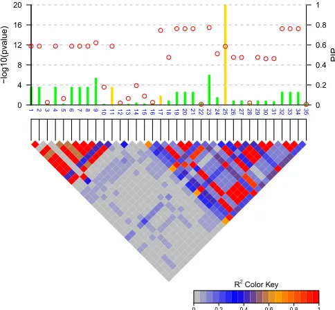
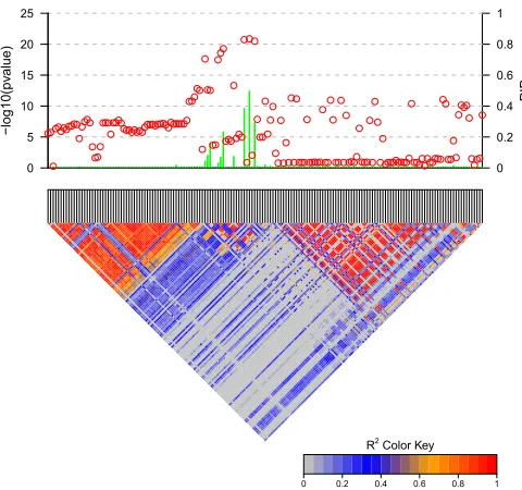
First we demonstrate the advantage of marginal PIPs over P-values in identifying candidate causal SNPs. Figure 1 shows the result of fine mapping on a simulated data set with 3 causal SNPs. PIPs were computed based on Bayes factors calculated from CAVIARBF. Circles represent the individual SNP-based P-value levels and lines represent the PIPs. The gold color indicates the true causal SNPs. The noncausal var-iant SNP23 had the smallestP-value, but this is purely due to high LD with the causal variant SNP17 and statisticalfl uctu-ation. The causal variant SNP25 did not achieve the smallest P-value, but it was correctly captured by the highest PIP. It seems that the causal variant SNP17 was ranked higher by P-values than by PIPs. However, from the perspective of the number of causal variants identified, ranking byP-values will include the first causal variant (SNP17) when 8 SNPs are selected, and ranking by PIPs will include on average 1 + 4/7 causal variants (SNP25 and SNP11) when 7 SNPs are selected (due to the same PIPs among SNP1, -2, -4, -6, -7, -8, and -11). If the correlation among SNPs is 1 or21, for ex-ample between the causal variant SNP11 and SNP1, -2, -4, -6, -7, -8, and -11, these SNPs will have the sameP-values and PIPs. To further distinguish them, extra information, such as functional annotation, may be helpful.

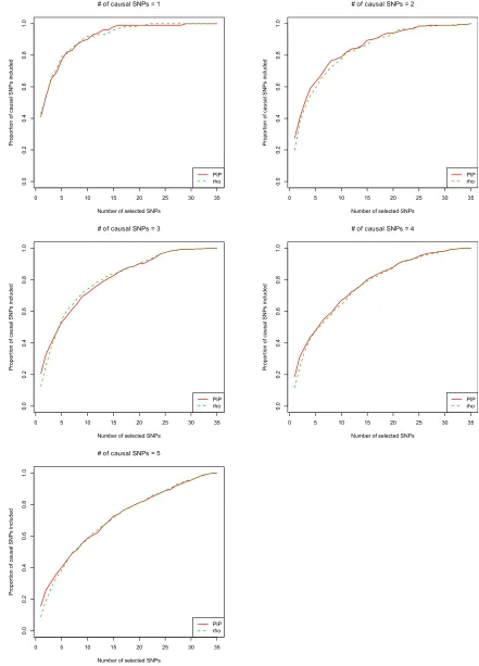
Proportion of causal SNPs included by different methods

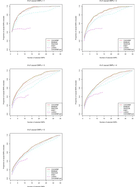
Figure 2 shows the proportion of causal SNPs included for different numbers of selected SNPs in 100 simulated data sets with quantitative traits. CAVIARBF, BIMBAM, and PAINTOR all use PIPs to rank SNPs and select the top SNPs. CAVIARBF and BIMBAM had similar performance as ex-pected. Note that this similar performance does not require a very large sample size, e.g., 2000 here. Similar perfor-mance between CAVIARBF and BIMBAM was also observed when the sample size was 200 (data not shown). When there was only 1 causal SNP, CAVIARBF, BIMBAM, and PAINTOR had similar performance. However, when there was.1 causal SNP, CAVIARBF and BIMBAM showed better performance than PAINTOR. One reason may be that PAIN-TOR uses the observed test statistics as the true underlying effect size, and therefore it does not account for the uncer-tainty of the effect size. On the other hand, CAVIARBF and BIMBAM incorporate the uncertainty by averaging (integrat-ing) over the prior distributions of effect sizes. ENET had better performance than LASSO, but worse performance than CAVIARBF, BIMBAM, or PAINTOR. One reason for the worst performance of LASSO is that when a causal var-iant has correlation 1 or 21 with other noncausal variants, LASSO will pick only one and ignore the rest. If the causal variant is not picked, it will not have the chance to be picked again as the model size increases. As expected, CAVIARBF had better performance than CAVIARBF(ref) because of us-ing the true correlation matrix. However, CAVIARBF(ref)

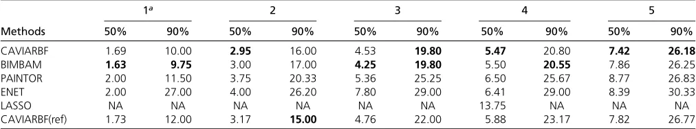
still had good performance, and in general it was the third best method among all compared, following CAVIARBF and BIMBAM. The differences among methods were small when only few SNPs were selected, but the differences became larger in the middle, i.e., around half of the total number of SNPs, and were small again when almost all SNPs were selected. In each plot, if weﬁx the proportion of causal SNPs included (they-axis), we can compare the number of SNPs needed to reach that proportion, which is linearly interpo-lated based on the discrete numbers on the x-axis. Table 1 shows the average number of SNPs needed to include 50% or 90% of the causal SNPs among 100 simulated data sets. For example, when there were 3 causal SNPs, to include 90% of the causal SNPs, the average numbers of SNPs needed were 19.80 for CAVIARBF and BIMBAM, 25.25 for PAINTOR, 29.00 for ENET, and 22.00 for CAVIARBF(ref). The results were similar for binary traits, which are shown in

Figure S1andTable S1.

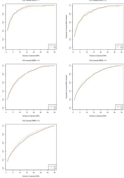
Choices and robustness ofsa

For both CAVIARBF and BIMBAM, we needed to specifysa:

We found that the results were robust with different values of sa: Figure 3 shows the result of CAVIARBF on quantitative

traits by settingsato 0.1 and 0.4, which are common values

used from BIMBAM’s manual. The results were similar except for the case ofﬁve causal SNPs where settingsato 0.4 showed

Pairwise LD, P values and marginal posterior inclusion probabilities (PIPs)

1 2 3 4 5 6 7 8 9 10 11 12 13 14 15 16 17 18 19 20 21 22 23 24 25 26 27 28 29 30 31 32 33 34 35

R2_{Color Key}

0 0.2 0.4 0.6 0.8 1

0 0.2 0.4 0.6 0.8 1 PIP 0 4 8 12 16 20 − log10(pv alue)

(8)

(9)

a slightly better performance. Similar robustness was observed for binary traits (seeFigure S2). Another possible way to choose sa is to try several values and choose the one that

maximizes the likelihood of the given data. This is similar to the empirical Bayesian method. When computation time is not an issue, this may result in a more robust and improved performance.

r-Level conﬁdence set vs. marginal PIP

Even though choosing SNPs with the top marginal PIPs maximizes the expected number of causal SNPs, we want to compare this criterion with the r-level confidence set, as proposed in CAVIAR (Hormozdiari et al. 2014). Figure 4 and Figure S3 show the results for quantitative traits and binary traits, respectively. In general, the results from the two different selection criteria were very similar if the num-ber of selected SNPs was not too small. Specifically, it seems that selecting SNPs using marginal PIPs usually had better performance than ther-level confidence set at thefirst few steps. This is reasonable. Take thefirst step, for example. For each candidate SNP, the r-level confidence set considers only the causal model that is composed of the candidate SNP. In contrast, the marginal PIP considers all models that include the candidate SNP. The marginal PIP gives the likeli-hood that a candidate SNP is causal among all possible causal models, while the r-level confidence set gives the likelihood that a candidate SNP is causal, assuming there is only one causal SNP. Obviously, marginal PIP is what we want when there are multiple causal SNPs. Interestingly, when the number of selected SNPs was large enough, e.g., no less than five, the two methods showed similar results. Given that the marginal PIP is much easier and faster to compute and ranking by PIP maximizes the expected num-ber of causal variants, we recommend using itfirst. In our implementation, we still provide an option to calculate the r-level confidence set if the user wants to have an estimate of the probability that all causal SNPs have been included in each selection step. The forward stepwise selection to con-struct a r-level confidence set may have some advantages when there are interactions among causal SNPs. There might be more flexible stepwise procedures that allow previously selected SNPs to be removed from the model or swapped with others. These could be a topic for further study.

Estimated probability ofr-level conﬁdence set

In this section we estimate the probability of including all causal SNPs. Figure 5 shows the estimated probability and the distribution (boxplot) of the number of selected SNPs for quantitative traits. The nominal rlevel was set to 0.9. For CAVIARBF and BIMBAM, when the number of causal SNPs was no more than three, the estimated probability was larger than the nominal level, which means more SNPs than needed were selected. When the number of causal SNPs was

five, the estimated probability was 0.7, lower than the nominal level. This inaccurate r-level estimation was be-cause we used a model that assumed the expected number of causal SNPs in the data was one, much smaller thanfive. Therefore in real data analysis, even though the estimated probability rfor each SNP set can usually give a rough in-dication of the probability of including all causal SNPs, it should be interpreted with some caution. For ENET and LASSO, we first used cross-validation to select the best parameters and then used the selected parameters to build the best model, using the full data. It was obvious that both ENET and LASSO cannot guarantee a high probability of including all causal SNPs based on the best model built from the data, even though the number of the selected SNPs was much smaller than those from CAVIARBF and BIMBAM. For binary traits, similar patterns were observed (seeFigure S4). The results show that CAVIARBF or BIMBAM selected more SNPs than ENET or LASSO but achieved a higher probability of including all causal SNPs. We questioned whether this was due to the high correlation between SNPs in the simulated data set or other factors. To answer this, we simulated data sets with quantitative traits where SNPs were independent from each other. Results are shown in

Figure S5. For data sets with less than five causal SNPs, CAVIARBF and BIMBAM selected more SNPs than needed; i.e., the reported level of confidence was conservative even in the case of independent SNPs. We think that this is due to the uncertainty on the number of causal SNPs. For example, for the data set with only one causal SNP, allowing a maxi-mum of five causal SNPs with CAVIARBF and BIMBAM may also take into account other possible small effects, resulting in more SNPs needed to reach a nominal level than that assuming only one causal SNP. For data sets with

ﬁve causal SNPs, which was also the maximal number of

Table 1 Average number of SNPs needed to include 50% and 90% causal SNPs among 100 simulated data sets under different numbers of causal SNPs for continuous traits

Methods

1a 2 3 4 5

50% 90% 50% 90% 50% 90% 50% 90% 50% 90%

CAVIARBF 1.69 10.00 2.95 16.00 4.53 19.80 5.47 20.80 7.42 26.18

BIMBAM 1.63 9.75 3.00 17.00 4.25 19.80 5.50 20.55 7.86 26.25

PAINTOR 2.00 11.50 3.75 20.33 5.36 25.25 6.50 25.67 8.77 26.83

ENET 2.00 27.00 4.00 26.20 7.80 29.00 6.41 29.00 8.39 30.33

LASSO NA NA NA NA NA NA 13.75 NA NA NA

CAVIARBF(ref) 1.73 12.00 3.17 15.00 4.76 22.00 5.88 23.17 7.82 26.77

a_{The number of causal SNPs in the data. The smallest number for each column is in boldface type. NA: data not available for the calculation. CAVIARBF(ref): CAVIARBF with}

(10)

(11)

(12)

(13)

causal SNPs allowed in the analysis, most of the time CAVIARBF and BIMBAM selected exactly theﬁve causal SNPs because no extra small effects needed to be considered. This number was also lower than that from ENET or LASSO. The single rlevel of a candidate set provides limited information about the selected SNPs; another informative way is to look at the marginal PIPs, as shown inFigure S6. There were three causal SNPs in the data set, which correspond to the marginal PIPs close to 1 (gold lines). Compared to Figure 1, the pattern here is much simpler and reﬂects the independence among SNPs.

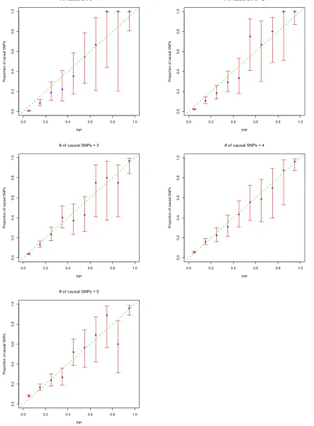
Calibration of the PIPs

PIPs are more useful if they are well calibrated. To assess the accuracy of estimated PIPs, following Guan and Stephens (2011), we put SNPs into 10 bins according to their PIPs. Each bin’s width was 0.1. We chose 10 bins instead of 20 due to the small number of counts in some bins. Then we compared the proportion of causal SNPs in each bin with the center PIP of that bin. Figure 6 shows the plots using quan-titative traits. Except those bins with very large conﬁdence intervals, due to small total counts in the bins, in general the points lie near the diagonal line. This indicates that the PIPs are reasonably calibrated. Therefore PIPs can be used not only to rank SNPs, but also as an indication of the expected number of SNPs in the candidate set. Similar results for bi-nary traits are shown inFigure S7.

Time cost

For CAVIARBF and BIMBAM, the time cost depends on the total number of SNPspand the maximal number of causal SNPs allowed, l. The total number of causal models is

Pl i¼0

p i

;which is dominated by the combinatorial term

p l

. Becauseðp=lÞl#

p l

#pl₌_l!_#_ðð_p_e_Þ=_l_Þl_;

if weﬁxp,

for smalllmuch less thanp,

p l

increases approximately exponentially with respect to l. If we ﬁx l, it is bounded above by a polynomial complexity of degreel. For a reason-able running time, lis usually small,e.g., no more than 5. The total number of SNPspcan be relatively larger. Figure 7 shows the actual time cost for quantitative traits with differ-ent p when l = 3, 4, and 5. ENET was based on the R packageelastic netwith 10-fold cross-validation and LASSO was based on the R packagelars. For PAINTOR, we set the number of iterations to two because after that the likelihood changed little. CAVIARBF takes about quarter to

one-ﬁfth of the time of BIMBAM. For example forl= 3, when the number of SNPs was 200, the time was44 sec for CAVIARBF and 229 sec for BIMBAM. CAVIARBF was slower than PAINTOR when p ,200 but faster than PAINTOR when pbecame larger. This is because PAINTOR always uses all the SNPs in the computation of the likelihood for each model while CAIVARBF uses only those SNPs included in each model to calculate the likelihood.

Application of methods

To compare different methods on real data, we used two GWAS cohorts designed to identity genetic variants associated with variation in smallpox vaccine-induced immune responses. The phenotype of interest is vaccinia virus-induced IFN-a pro-duction detected in peripheral blood mononuclear cells (PBMCs) fromfirst-time recipients of smallpox vaccine. More details about the study cohorts can be found in Ovsyannikova et al.(2011, 2012, 2014) and Kennedyet al.(2012). Thefirst cohort, called the San Diego cohort, included 1076 recipients of Dryvax, of which 488 were Caucasian and had the IFN-a outcome available and genotypes measured by the Illumina HumHap 550 platform. Genotypes were imputed using IM-PUTE2 (Howieet al.2009) with the reference panel from the 1000 Genomes Phase 1 haplotypes. The second cohort, called the U.S. cohort, included 1058 recipients of ACAM2000, of which 734 were Caucasian and 713 of them had the IFN-a outcome available. The genotypes were measured by the Omni 2.5S genome-wide SNP chip. For the U.S. cohort (mainly Caucasian), the European (EUR) population was used as the reference panel. For the San Diego cohort (a mix of different race and ethnic groups), the EUR, East Asian (ASN), African (AFR), and Admixed American (AMR) pop-ulations were used as the reference panel. For both cohorts, the analyses were restricted to Caucasians. For the U.S. cohort, the phenotype was regressed on the following covariates: gender, time from immunization to blood draw, vaccination date, immune assay batch, and thefirst principal component to adjust for potential population stratification. For the San Diego cohort, the phenotype was regressed on the following covariates: date of IFN-aassay, date of blood draw, shipping temperature of the sample, site the sample was drawn from, and the second principal component (the first is not in-cluded because it is not significant). The residuals from these regressions were used as the analysis phenotype. We focused on a region of chromosome 5 where multiple SNPs reached the genome-wide significance level of 531028for both cohorts. We chose the region based on a cluster of peak signals and included100 SNPs on both sides of the target region. Furthermore, SNPs with minor allele frequency (MAF),5% in each cohort were removed, leaving 167 SNPs in the U.S. cohort and 200 SNPs in the San Diego cohort for

ﬁne-mapping analysis. The mode of posterior probabilities from IMPUTE2 for each SNP averaged over all individuals was .0.8, and the overall average across all SNPs was

.0.97. We set the maximal number of causal SNPs to 3 and 4. Because they showed similar results, there was no need to use a larger maximal number of causal SNPs. We present the results corresponding to a maximum of 4 causal SNPs. For BIMBAM and CAVIARBF, we set sa to 0.1 and

used the original SNP matrix (not scaled) in the model. The prior probability of being causal for each SNP is set to 1/m, wheremis the number of SNPs.

The overall Bayes factor BFðMg:M0Þ measures the

(14)

(15)

For the U.S. cohort, it was 2.531013_{, which is very strong}

evidence favoring the model that there is at least one causal variant. For the San Diego cohort it was 8.13107_{, which is}

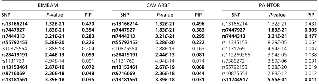
much smaller than the U.S. cohort but is still suggestive even if we use a very conservative prior, say 1027. One obvious reason for the smaller Bayes factor is the smaller sample size in the San Diego cohort. The overall evidence of the region also makes the prior assumption of 1 expected causal SNP in the region reasonable. Figure 8 shows the PIPs from CAVIARBF on the U.S. cohort. PIPs of many SNPs in the plot are very small and can be excluded from the candidate causal set. Some of these excluded SNPs have P-values

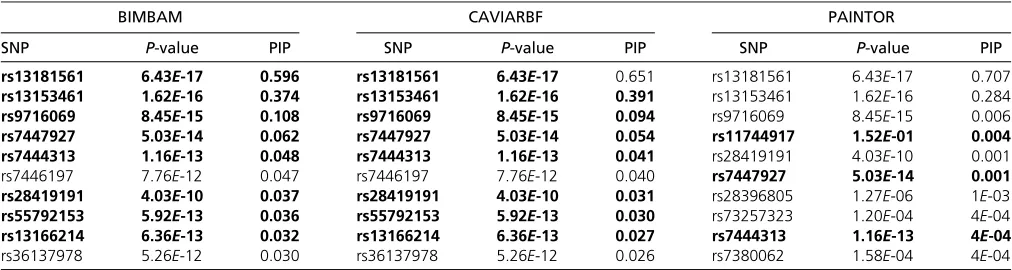
,10210; however, this is likely due to their being in close LD with causal variants. PIPs from BIMBAM and PAINTOR on the U.S. cohort are shown in Figure S8and Figure S9, respectively. As in the simulation results, CAVIARBF and BIMBAM showed similar results. PAINTOR identified the same top 3 SNPs as CAVIARBF and BIMBAM; however, the pattern of the remaining SNPs was different. CAVIARBF and BIMBAM still included other SNPs with relatively large PIPs, while PAINTOR-selected SNPs had very small PIPs. This may be due to treating afixed or estimated noncentrality param-eter (effect size) as the true value in PAINTOR, while in CAVIARBF and BIMBAM a prior distribution of the effect size is assumed. Similar patterns are shown on the San Diego cohort (see Figure S10,Figure S11, andFigure S12). The top 10 SNPs from each method on two cohorts are presented in Table 2 and Table 3. For both cohorts, CAVIARBF and BIMBAM identified the same top 10 SNPs and ranked them identically. PIPs are similar between BIMBAM and CAVIARBF. On the other hand, PAINTOR included some different SNPs. Some of the top 10 SNPs selected by BIMBAM and CAVIARBF were ranked.50 by PAINTOR. Next we ex-amined the number of SNPs shared in the top 10 SNPs picked by each method between two cohorts. These SNPs are indi-cated in boldface type in Table 2 and Table 3. For BIMBAM and CAVIARBF, 8 of 10 SNPs are shared while there are only 3 SNPs shared for PAINTOR. We also found that one of the shared SNPs picked by PAINTOR seems counterintuitive. This SNP (rs11744917) was ranked 10th with aP-value of 0.555 in the U.S. cohort, and ranked 4th with aP-value of 0.152 in the San Diego cohort. The same SNP was ranked 47

Figure 7 Time cost of different methods. Different maximal numbers of causal SNPs are tested for CAVIARBF, BIMBAM, and PAINTOR. They-axis is on a log10 scale. Thex-axis shows the total number of SNPs in the input data.

Pairwise LD, P values and marginal posterior inclusion probabilities (PIPs)

R2_{Color Key}

0 0.2 0.4 0.6 0.8 1

PIP

0 5 10 15 20 25

−

log10(pv

alue)

(16)

by CAVIARBF and 48 by BIMBAM in the U.S. cohort and 49 by CAVIARBF and 57 by BIMBAM in the San Diego cohort. Because no functional study has been performed yet to verify the underlying causal variants, no conclusion can be made on the performance of different methods. However, the PIP pat-terns and the sharing of the top 10 SNPs may shed some light on the characteristics of different methods. One advantage of CAVIARBF is the use of summary statistics. We also tried to use only the z test statistics and estimated LD pattern (the correlation coefﬁcient matrix among SNPs) from the 1000 Genomes Project, using EUR samples.Figure S13shows the PIPs and LD plots on the U.S. cohort. Compared to the result from using the LD matrix calculated from the U.S. cohort, even though there are some distortions, the general patterns are similar. As the numbers of samples in the study and in the reference panel increase, assuming a good match of ancestry background, the estimation of the correlation matrix will be-come more stable and accurate. Therefore, we anticipate the PIPs from using only theztest statistic and correlations from reference panels will become more accurate in studies with large samples.

Discussion

By proving that BIMBAM and CAVIAR are approximately equivalent, we provided a Bayesian framework offine map-ping using marginal test statistics and correlation coeffi -cients among SNPs. We also provided a fast implementation, CAVIARBF. Compared to CAVIAR, CAVIARBF has the follow-ing main advantages: (1) it is much faster largely because it uses only the SNPs in each causal model to calculate Bayes factors; (2) it unifies thefine-mapping and association tests in a consistent Bayesian framework; and (3) it is Bayes factor centered, so the output Bayes factors can be used for other analysis,e.g., calculating the evidence of at least 1 causal SNP in the region. Our simulation showed that the performances of BIMBAM and CAVIARBF are almost the same, as expected. CAVIARBF had better performance than PAINTOR, which has been shown to be a very competitive method to other fi ne-mapping methods (Kichaevet al.2014). Our implementation is about four tofive times as fast as BIMBAM. Application to

real data showed that BIMBAM and CAVIARBF identiﬁed the same top 10 SNPs with the same ranking. PAINTOR identiﬁed 3 of the same top 10 SNPs (those with large PIPs) as BIMBAM and CAVIARBF. BIMBAM and CAVIARBF may be more con-sistent than PAINTOR in prioritizing causal SNPs because 8 of the 10 top SNPs were shared between two cohorts on the same phenotype.

The approximate equivalence between BIMBAM using the full dataðy; XÞand CAVIAR/CAVIARBF using only the marginal test statistics and the correlation coefﬁcient matrix

ðz;SxÞcan also be explained in terms of sufﬁcient statistics.

For example, for quantitative traits, let D1¼ ðy; XÞ: If we

assume the variance of y is known, we can equivalently write the inputðz; SxÞasD2 ¼ ðXTy; XTXÞ:The likelihood

function lðy; XjbÞ ¼pðXÞpðyjX;bÞ: The conditional proba-bility pðyjX;bÞ depends only on ðy2XbÞTðy2XbÞ ¼yT_y_þ

bT

XT_Xb₂₂_bT

XT_y_;_{where the part involving both}

param-eter b and data is bTXT_Xb₂₂_bT

XT_y_: _Therefore _D 2¼ ðXT_y_; _XT_X_Þ_{is the suf}_ﬁ_{cient statistic for the model parameter}

b. Then it can be shown that the Bayes factor depends only on the sufﬁcient statistics. More details of proving the equiv-alence for binary traits are given inFile S1.

The analytic Bayes factor is also derived in Wen (2014). For example, Equation 3 can be derived from equation 9 in Wen (2014), even though the marginal test statistics are not used directly. In Wen (2014), it also proves the ap-proximation when the error variance 1=tis unknown. Sim-ilar derivations could be applied for the marginal test statistics.

All derivations assume no covariates in the model. When there are covariates, for quantitative traits, as suggested in the manual of BIMBAM, we can regress the trait on all covariatesﬁrst and use the residual as the new trait. Because CAVIARBF needs only the input of marginal test statistics, a natural way is to calculate the test statistic for each SNP adjusted for other covariates. This method can be applied to both quantitative traits and binary traits. Further analysis is needed to fully validate the effectiveness of this handling of covariates.

For a well-powered GWAS, there are usually multiple loci with potential causal variants for further ﬁne mapping.

Table 2 Top 10 variants ranked by PIPs from different methods and the correspondingP-values on the U.S. cohort

BIMBAM CAVIARBF PAINTOR

SNP P-value PIP SNP P-value PIP SNP P-value PIP

rs13166214 1.32E-21 0.470 rs13166214 1.32E-21 0.496 rs13166214 1.32E-21 0.431 rs7447927 1.83E-21 0.354 rs7447927 1.83E-21 0.383 rs7447927 1.83E-21 0.305 rs7444313 3.21E-21 0.283 rs7444313 3.21E-21 0.295 rs7444313 3.21E-21 0.177 rs55792153 5.28E-20 0.226 rs55792153 5.28E-20 0.232 rs113451531 8.29E-05 0.064 rs10875554 2.88E-13 0.204 rs10875554 2.88E-13 0.163 rs1131769 4.94E-14 0.047 rs28419191 2.44E-13 0.099 rs28419191 2.44E-13 0.081 rs112269266 3.94E-05 0.038

rs1131769 4.94E-14 0.091 rs1131769 4.94E-14 0.074 rs7380272 3.59E-06 0.031

rs13153461 2.67E-19 0.072 rs13153461 2.67E-19 0.068 rs55792153 5.28E-20 0.019 rs9716069 2.36E-18 0.048 rs9716069 2.36E-18 0.044 rs10875554 2.88E-13 0.012 rs13181561 3.39E-18 0.035 rs13181561 3.39E-18 0.031 rs11744917 5.55E-01 0.011

(17)

Usually these loci can be assumed to be independent of one another. In this case we can ﬁrst doﬁne mapping of each locus and then pool all PIPs of the SNPs in these loci together and choose the top k SNPs as recommended in Kichaevet al.(2014).

We considered only common variants in this study. For common variants, it might be practical to assume a maximal number of causal variants in a locus,e.g., no more thanfive. When the maximal number of causal SNPs in a model is lim-ited, all possible models can be enumerated exhaustively in a reasonable time if the number of SNPs in a locus is not too large. This is different from typical Bayesian methods where sampling methods, such as MCMC, are often used to sample models from the model space (Wilsonet al.2010; Guan and Stephens 2011). The sampling methods would be useful if more thanfive causal variants are expected in a large region with high LD among SNPs. On the other hand, if a large region can be divided into multiple uncorrelated or weakly correlated regions, we can perform fine mapping in each region, and then combine the results together. For rare variants, there may be many rare causal variants in a region, and therefore sampling methods may be required to explore the model space. Some Bayesian-based methods have been proposed for rare variants, such as in Quintanaet al.(2011, 2012).

Because the Bayesian framework can also answer the association question, in principle the proposed method can be used for genome-wide association scans. Because of the consideration of multiple causal SNPs in a region, it may achieve higher power to discover the association regions than the traditional individual SNP-based test. This has already been demonstrated in Wilson et al. (2010) and Guan and Stephens (2011), using the true positive vs. false positives plot. However, the time cost may be much larger compared to that of individual SNP-based tests. Further reduction in time cost will be helpful for this application.

We assumed the effects of multiple causal SNPs are additive (for binary traits, additive on logit scale) and the effect of each causal genotype is additive. We believe these assumptions are reasonable for most cases. In principle, the dominance effect of each SNP can be included by adding an extra column indicating the genotype heterozygosity as

implemented in BIMBAM. How to include a nonadditive combination of effects from multiple causal SNPs will be an interesting topic of further study.

We assumed that functional annotations of SNPs are not included in fine mapping. As pointed out in Kichaev et al. (2014) and Pickrell (2014), a large amount of annotation information of genomic elements has been generated, such as the Encyclopedia of DNA Elements (ENCODE Project Consortium 2012). Including informative functional annota-tions into fine-mapping analysis will further increase the chance to filter out the underlying causal variants (Quintana and Conti 2013; Kichaevet al.2014; Pickrell 2014). In princi-ple, the same EM algorithm proposed in Kichaevet al.(2014) can be applied to extend our method to handle functional annotations. We leave this as a future direction to pursue.

Acknowledgments

We thank two reviewers for helpful discussion and sugges-tions. This research was supported by the U.S. Public Health Service, National Institutes of Health, contract grant no. GM065450 and by federal funds from the National Institute of Allergies and Infectious Diseases, National Institutes of Health, Department of Health and Human Services, under contract no. HHSN272201000025C. The content is solely the responsibility of the authors and does not necessarily repre-sent the ofﬁcial views of the National Institutes of Health.

Literature Cited

Abecasis, G. R., A. Auton, L. D. Brooks, M. A. DePristo, R. M. Durbin

et al., 2012 An integrated map of genetic variation from 1,092 human genomes. Nature 491: 56–65.

Altshuler, D. M., R. A. Gibbs, L. Peltonen, E. Dermitzakis, S. F. Schaffner et al., 2010 Integrating common and rare genetic variation in diverse human populations. Nature 467: 52–58. Armitage, P., 1955 Tests for linear trends in proportions and

fre-quencies. Biometrics 11: 375–386.

Durrant, C., K. T. Zondervan, L. R. Cardon, S. Hunt, P. Deloukas

et al., 2004 Linkage disequilibrium mapping via cladistic analysis of single-nucleotide polymorphism haplotypes. Am. J. Hum. Genet. 75: 35_–43.

Table 3 Top 10 variants ranked by PIPs from different methods and the correspondingP-values on the San Diego cohort

BIMBAM CAVIARBF PAINTOR

SNP P-value PIP SNP P-value PIP SNP P-value PIP

rs13181561 6.43E-17 0.596 rs13181561 6.43E-17 0.651 rs13181561 6.43E-17 0.707 rs13153461 1.62E-16 0.374 rs13153461 1.62E-16 0.391 rs13153461 1.62E-16 0.284 rs9716069 8.45E-15 0.108 rs9716069 8.45E-15 0.094 rs9716069 8.45E-15 0.006 rs7447927 5.03E-14 0.062 rs7447927 5.03E-14 0.054 rs11744917 1.52E-01 0.004 rs7444313 1.16E-13 0.048 rs7444313 1.16E-13 0.041 rs28419191 4.03E-10 0.001

rs7446197 7.76E-12 0.047 rs7446197 7.76E-12 0.040 rs7447927 5.03E-14 0.001

rs28419191 4.03E-10 0.037 rs28419191 4.03E-10 0.031 rs28396805 1.27E-06 1E-03 rs55792153 5.92E-13 0.036 rs55792153 5.92E-13 0.030 rs73257323 1.20E-04 4E-04 rs13166214 6.36E-13 0.032 rs13166214 6.36E-13 0.027 rs7444313 1.16E-13 4E-04 rs36137978 5.26E-12 0.030 rs36137978 5.26E-12 0.026 rs7380062 1.58E-04 4E-04

(18)

ENCODE Project Consortium, 2012 An integrated encyclopedia of DNA elements in the human genome. Nature 489: 57–74. Faye, L. L., M. J. Machiela, P. Kraft, S. B. Bull, and L. Sun,

2013 Re-ranking sequencing variants in the post-GWAS era for accurate causal variant identiﬁcation. PLoS Genet. 9: e1003609.

Guan, Y., and M. Stephens, 2008 Practical issues in imputation-based association mapping. PLoS Genet. 4: e1000279. Guan, Y. T., and M. Stephens, 2011 Bayesian variable selection

regression for genome-wide association studies and other large-scale problems. Ann. Appl. Stat. 5: 1780_–1815.

Harville, D. A., 2008 Matrix Algebra from a Statistician_’s Perspec-tive. Springer-Verlag, New York.

Hindorff, L., J. MacArthur, J. Morales, H. Junkins, P. Hall et al., 2014 A Catalog of Published Genome-Wide Association Studies. Available at: www.genome.gov/gwastudies. Accessed: Decem-ber 23, 2014.

Hormozdiari, F., E. Kostem, E. Y. Kang, B. Pasaniuc, and E. Eskin, 2014 Identifying causal variants at loci with multiple signals of association. Genetics 198: 497–508.

Howie, B. N., P. Donnelly, and J. Marchini, 2009 Aﬂexible and accurate genotype imputation method for the next generation of genome-wide association studies. PLoS Genet. 5: e1000529. Kennedy, R. B., I. G. Ovsyannikova, V. S. Pankratz, I. H. Haralambieva,

R. A. Vierkant et al., 2012 Genome-wide analysis of polymor-phisms associated with cytokine responses in smallpox vaccine recipients. Hum. Genet. 131: 1403–1421.

Kichaev, G., W. Y. Yang, S. Lindstrom, F. Hormozdiari, E. Eskin

et al., 2014 Integrating functional data to prioritize causal variants in statistical _ﬁne-mapping studies. PLoS Genet. 10: e1004722.

Liang, K. Y., and Y. F. Chiu, 2005 Multipoint linkage disequilib-rium mapping using case-control designs. Genet. Epidemiol. 29: 365–376.

Maller, J. B., G. McVean, J. Byrnes, D. Vukcevic, K. Palin et al., 2012 Bayesian reﬁnement of association signals for 14 loci in 3 common diseases. Nat. Genet. 44: 1294–1301.

Minichiello, M. J., and R. Durbin, 2006 Mapping trait loci by use of inferred ancestral recombination graphs. Am. J. Hum. Genet. 79: 910–922.

Morris, A. P., J. C. Whittaker, and D. J. Balding, 2002 Fine-scale mapping of disease loci via shattered coalescent modeling of genealogies. Am. J. Hum. Genet. 70: 686–707.

Ovsyannikova, I. G., R. A. Vierkant, V. S. Pankratz, R. M. Jacobson, and G. A. Poland, 2011 Human leukocyte antigen genotypes in the genetic control of adaptive immune responses to smallpox vaccine. J. Infect. Dis. 203: 1546_–1555.

Ovsyannikova, I. G., R. B. Kennedy, M. O’Byrne, R. M. Jacobson, V. S. Pankratzet al., 2012 Genome-wide association study of antibody response to smallpox vaccine. Vaccine 30: 4182–4189. Ovsyannikova, I. G., V. S. Pankratz, H. M. Salk, R. B. Kennedy, and G. A. Poland, 2014 HLA alleles associated with the adaptive immune response to smallpox vaccine: a replication study. Hum. Genet. 133: 1083–1092.

Pickrell, J. K., 2014 Joint analysis of functional genomic data and genome-wide association studies of 18 human traits. Am. J. Hum. Genet. 94: 559–573.

Quintana, M. A., and D. V. Conti, 2013 Integrative variable selec-tion via Bayesian model uncertainty. Stat. Med. 32: 4938–4953. Quintana, M. A., J. L. Berstein, D. C. Thomas, and D. V. Conti, 2011 Incorporating model uncertainty in detecting rare var-iants: the Bayesian risk index. Genet. Epidemiol. 35: 638–649. Quintana, M. A., F. R. Schumacher, G. Casey, J. L. Bernstein, L. Li

et al., 2012 Incorporating prior biologic information for high-dimensional rare variant association studies. Hum. Hered. 74: 184–195.

Scott, J. G., and J. O. Berger, 2010 Bayes and empirical-Bayes multiplicity adjustment in the variable-selection problem. Ann. Stat. 38: 2587–2619.

Servin, B., and M. Stephens, 2007 Imputation-based analysis of association studies: candidate regions and quantitative traits. PLoS Genet. 3: e114.

Stephens, M., and D. J. Balding, 2009 Bayesian statistical methods for genetic association studies. Nat. Rev. Genet. 10: 681–690. Su, Z., J. Marchini, and P. Donnelly, 2011 HAPGEN2: simulation

of multiple disease SNPs. Bioinformatics 27: 2304_–2305. Tibshirani, R., 1996 Regression shrinkage and selection via the

Lasso. J. R. Stat. Soc. B 58: 267_–288.

Waldron, E. R., J. C. Whittaker, and D. J. Balding, 2006 Fine mapping of disease genes via haplotype clustering. Genet. Epi-demiol. 30: 170_–179.

Wen, X., 2014 Bayesian model selection in complex linear systems, as illustrated in genetic association studies. Biometrics 70: 73_–83. Wilson, M. A., E. S. Iversen, M. A. Clyde, S. C. Schmidler, and J. M. Schildkraut, 2010 Bayesian model search and multilevel infer-ence for Snp association studies. Ann. Appl. Stat. 4: 1342–1364. Zollner, S., and J. K. Pritchard, 2005 Coalescent-based association mapping andﬁne mapping of complex trait loci. Genetics 169: 1071–1092.

Zou, H., and T. Hastie, 2005 Regularization and variable selection via the elastic net. J. R. Stat. Soc. Ser. B Stat. Methodol. 67: 301–320.

(19)

GENETICS

Supporting Information

www.genetics.org/lookup/suppl/doi:10.1534/genetics.115.176107/-/DC1

Fine Mapping Causal Variants with an Approximate

Bayesian Method Using Marginal Test Statistics

Wenan Chen, Beth R. Larrabee, Inna G. Ovsyannikova, Richard B. Kennedy, Iana H. Haralambieva, Gregory A. Poland, and Daniel J. Schaid

(20)

File S1

Approximate equivalence between BIMBAM and CAVIAR for binary traits

For binary traits, we use a logistic model as follows:

𝑙𝑜𝑔

𝑝(𝑦𝑖=1)

𝑝(𝑦𝑖=0)

= 𝛼 + ∑

𝑋

𝑖𝑗 𝑇

_𝛽

𝑗 𝑚

𝑗=1

, 𝑖 = 1, ⋯ , 𝑛

(A1)

where

𝑦

𝑖

is the phenotype of individual i; 1 indicates a case and 0 indicates a control.

𝑋

𝑖𝑗

is the same

additively coded genotype of individual i and SNP j as for the above quantitative traits. The model

parameters are

𝛼

and

𝛽 = (𝛽

1

, ⋯ , 𝛽

𝑚

)

𝑇

. The phenotype vector is

𝑦 = (𝑦

1

, … , 𝑦

𝑛

)

𝑇

. Again we assume

each column of X has mean 0 and variance 1, i.e.,

1

𝑛

∑

𝑋

𝑖𝑗 𝑛

𝑖=1

= 0,

_𝑛1

∑

𝑛𝑖=1

𝑋

𝑖𝑗2

= 1, 𝑗 = 1, 2, … , 𝑛

. Denote

the number of cases and controls by

𝑛

1

and

𝑛

2

, respectively. Let

𝑋̅ = (1

𝑛×1

, 𝑋), 𝛽̅ = (𝛼, 𝛽)

𝑇

, where

1

𝑛×1

means the

𝑛 × 1

vector of 1s. We assume a normal prior distribution for

𝛽̅

, i.e.,

𝛽̅~𝑁(0, 𝑣̅)

, where

𝑣̅

is a diagonal matrix with positive diagonal entries. Denote the first diagonal entry for

𝛼

by

𝜎

_𝛼2

, the rest of

the diagonal matrix by

𝑣

, the variance of

𝛽

. The null model is

𝛽 = 0

𝑚×1

, which is equivalent to setting

𝑣

to

0

𝑚×𝑚

, where

0

𝑚×1

is a

𝑚 × 1

vector of 0s, and

0

𝑚×𝑚

is a

𝑚 × 𝑚

matrix of 0s. The Bayes factor

comparing the full model with the null model is

𝐵𝐹 =

𝑝(𝑦, 𝑋̅|𝜎

𝛼2

, 𝑣)

𝑝(𝑦, 𝑋̅|𝜎

_𝛼2

_{, 𝑣 = 0}

𝑚×𝑚

)

,

where

𝑝(𝑦, 𝑋̅|𝜎

𝛼2

, 𝑣) = ∫ 𝑝(𝑦, 𝑋̅|𝛽̅)𝑝(𝛽̅|𝜎

𝛼2