Article
Visualization of the Strain-rate State of a Data Cloud:
Analysis of the Temporal Change of an Urban
Multivariate Description
Lorena Salazar-Llano1,3, Camilo Bayona-Roa2,3∗
1 Sustainability Measurement and Modeling Lab., Universitat Politecnica de Catalunya – Barcelona Tech,
Barcelona (Spain); E-Mail: [email protected] (L. S.-L.)
2 Universidad Nacional de Colombia, Bogotá (Colombia); E-Mail: [email protected] (C. B.-R.) 3 Centro de Ingeniería Avanzada, Investigación y Desarrollo – CIAID, Bogotá (Colombia)
1
2
3
4
5
6
7
8
9
10
11
12
13
* Correspondence:[email protected]
Abstract: Onechallengingproblemistherepresentationofthree-dimensionaldatasetsthatvary withtime.Thesedatasetscanbethoughasacloudofpointsthatgraduallydeforms. Butpoint-wise variationslackofinformationabouttheoveralldeformationpattern,andmoreimportantly,about the extreme deformation locations inside the cloud. Thepresent articleapplies a technique in computationalmechanicstoderivethestrain-ratestateofatime-dependentandthree-dimensional datadistribution,bywhichonecancharacterizeitsmaintrendsofshift.Indeed,thetensorialanalysis methodologyisabletodeterminetheglobaldeformationratesintheentiredataset.Withtheuseof thistechnique,onecancharacterizethesignificantfluctuationsinareducedmultivariatedescription ofanurbansystemandidentifythepossiblecausesofthosechanges:calculatingthestrain-ratestate ofaPCA-basedmultivariatedescriptionofanurbansystem,weareabletodescribetheclustering anddivergencepatterns betweenthedistrictsofthecityandtocharacterizethetemporalratein whichthosevariationshappen.
Keywords: dimensionality reduction; pattern identification; three-dimensional data-cloud; strain-rate;FiniteElementMethod(FEM);trajectoryvisualization
14
1. Introduction 15
One challenging problem in the data analysis is the representation of three-dimensional discrete 16
data [1]. This analysis becomes harder when a time-dependent change of the data takes place, 17
introducing a new temporal dimension. In the present article, we explore formal approaches to 18
quantify the temporal change of discrete three-dimensional data. Specifically, we build a methodology 19
to assess the transformation of a data cloud that is derived from aPrincipal Component Analysis(PCA): a 20
13-years span multivariate description in [2] that provides a reduced description of an urban system 21
given only by the first three principal components. Since the points represent an abstraction of an 22
urban system, one main goal is to understand the temporal variation of the multivariate description of 23
the districts in order to analyze the behavior of the overall city in the time-span. Our main hypothesis 24
is that these three-dimensional datasets can be though as a cloud of points that gradually deforms. 25
Still, the challenging issue is that deformation between consecutive times cannot be visualized 26
straightforwardly. There are some methods to overcome this difficulty. One is the vector plot 27
of three-dimensional displacements or velocities, that is typically used to visualize results in 28
Computational Mechanics applications [3–5]. In example, these are used in the Kinematic Visualization 29
of Motion in [6–10], but they are restricted to display relative motion among the data, and are not able 30
to identify the most dynamic regions of the dataset. Another is the Parallel Coordinate Technique that 31
successfully exhibits the temporal change of highly-dimensional statistical and information datasets 32
[11]. Yet, multi-dimensional data is typically segmented in two-dimensional subsets, like the Computer 33
Tomographic scans of medical imaging [1,12,13]. Furthermore, the previously mentioned methods are 34
not suitable when one aim to understand the patterns of diversification or conformation, which are 35
closely related to the temporal change of the differences between join data values: the maximum and 36
minimum magnitudes of variation and the evaluation of their direction can be significantly helpful 37
when one aims to identify differentiation patterns in the data [14]. Or the opposite, when one aims to 38
locate uniformity for a dataset which was previously differentiated. 39
The field of continuum mechanics provides a measure of the temporal variation of the distance 40
in between points: the Strain-Rate tensor(see, for instance, [15]). The continuum mechanics theory 41
-which arises from the classical Newtonian mechanics- analyzes the causes and effects of motion 42
for a deformable media composed by an infinite group of particles. When a continuous media is 43
being deformed in various directions at different rates, the strain-rate of a certain position in the 44
medium cannot be expressed by a scalar value solely. It cannot even be expressed by using a single 45
vector. Instead, the rate of deformation must be expressed by the rank-two strain-rate tensor with 46
its components determined by the positional derivatives along each spatial dimension. Hence, the 47
mathematical framework of tensors can determine exactly the deformation that is accumulated in a 48
certain position inside the medium -that is typically subjected to the imposition of displacements or 49
loads-. This tensor is commonly used to detail the amount of elastic energy in the physical descriptions 50
of multiple materials, like solids or fluids. See [16] for a complete mathematical exposition. Most of 51
those models are formulated as the product of a constitutive tensor and the strain-rate tensor, giving 52
the stress condition of the material that is balanced in the kinetic equations. In the present study, the 53
calculation of the strain-rate tensor is not related to the kinetics of any material, and thus, it can only 54
be a mathematical tool that supports the examination of the deformation rates given by the discrete 55
statistical data. 56
But the strain-rate tensor arises from the continuum assumption, and discrete displacements of 57
points rather than continuous distributions take place in the deformation of the data cloud. Typically, 58
the issue of applying derivatives to discrete displacements of points is solved by using several 59
approaches. Some statistical techniques use co-variance functions to represent directly the strain-rate 60
field (see e.g. [17]). But the common approach is to compute a continuous version of the displacement 61
-or velocity- field, so that, derivatives can be applied to the continuous displacements. Some methods, 62
in this line, have interpolated the discrete displacements by minimizing the residual -or distance-63
between the continuous interpolation and the discrete version [18]. Other interpolation techniques 64
weight the distance between an interpolated piece-wise continuous field and the discrete displacement 65
field, as in [19]. This method results in a minimization technique where a continuous strain-rate field 66
can be derived. In example, the piece-wise continuous field can be defined as to be splines, or as the 67
widely used linear polynomials in variational formulations [20]. These techniques have been applied 68
in earth science and medical imaging works [21–23], but also in the strain-rate calculation of geodetic 69
observations in [24,25]. 70
Another fundamental issue is the representation of the strain-rate state. One of the possible 71
techniques that can help to visualize the deformation rate of the dataset is to plot the main 72
components of the tensor usingStrain-rate diagrams, where concentrations of strain-rate patterns 73
can be displayed as vector fields (see for example the ones in geodetical observations of the earth’s 74
mantle [26–28]). The main drawback of strain-rate diagrams is that the strain-rate components are 75
visualized as the projection of three-dimensional vector fields into the two-dimensional framework, 76
and therefore, the third-dimension component is necessarily neglected. Another method, more suitable 77
to two-dimensional plots, is the contour graph of principal stresses, where the stress patterns in 78
structural elements [29,30] and tectonics [31] are visualized with continuous lines depending on the 79
stress magnitude. That method overcome the three-dimensional issue, but it does not give insights 80
trajectories of the stress principal components in separated plots, where the stress magnitude can be 82
colored in each trajectory line such that stress patterns are exhibited in a two-dimensional framework. 83
This last technique has been our preferred approach in order to visualize the principal strain-rate 84
patterns of the three-dimensional data cloud. 85
Since a robust methodology that describes the temporal change of the urban system -represented 86
by a multivariate dataset- has not been carried out before, we choose to perform a quantitative analysis 87
by including the strain-rate tensor as the fundamental metric. In this work, we calculate the strain-rate 88
state of the discrete dataset withouta prioriassuming the mechanisms by which the system experiences 89
transformation. In order to apply the continuum mechanics principles into the discrete dataset, we 90
use interpolation methods, such as the ones applied in discrete variational formulations (i.e. Finite 91
Element Methods(FEM), Particle Methods, Collocation Methods, Mesh-less methods, etc.). Specifically, 92
we derive the three-dimensional strain-rate tensor from a FEM interpolation of the discrete velocity 93
field, as demonstrated in previous works such as [32–34]. We include a methodology for visualizing 94
the main patterns of change in any time-dependent data cloud that can be used in a computational 95
(two-dimensional) framework. It is based on the family of curves that are instantaneously tangent to 96
theextensionandcontractioncomponents of the strain-rate tensor: the so-calledtrajectorycurves of the 97
continuum mechanics field [15]. These help to overcome the three-dimensional representation problem, 98
since separated in several plots -one for each principal component-, demonstrate the magnitude and 99
orientations of the strain-rate patterns in a two-dimensional plot. 100
The remaining parts of this document are organized as follows. In Section2the methodology to 101
compute the discrete version of the strain-rate tensor is presented. Since the main problem involves 102
the calculation of the derivatives of discontinuous -discrete- velocities, we extensively review the 103
numerical techniques that are adopted to overcome this difficulty and the ones which are used for 104
visualizing the strain-rate patterns. Next, in Section3, we present the application of the methodology 105
to the case study -the urban system of Barcelona- by deriving its strain-rate state and visualizing its 106
main strain-rate patterns, meaning the city’s environmental, social and economic change. Finally, in 107
Section4some conclusions of the proposed methodology close this article. 108
2. Methods 109
We begin this section with a review of the strain-rate tensor calculation provided a discrete 110
three-dimensional data cloud. For doing so, the formal problem of the time-dependent dataset is 111
introduced first. Then, we explain the numerical techniques that transform the discrete dataset into 112
a mathematical framework by which the strain-rate tensor can be computed. Most of the ideas rely 113
on the geometrical analysis of the discrete dataset by computing the spatial discretization of the 114
dataset into geometric elements through aDelaunay Triangulation. After doing that, the computation 115
of the strain-rate is performed with a FEM interpolation of the velocity field. Finally, we address the 116
eigen-problemfor the strain-rate tensor, such that the solution of the eigenvalues, and the corresponding 117
eigenvectors, gives the extrema strain-rates at each finite element. The flow chart diagram of this 118
methodology is represented in Fig.1, including the main outputs that result at each step. The extended 119
explanation is developed along this section. 120
2.1. Time-dependent three-dimensional dataset 121
Since the main objective of this work is to reveal the temporal transformation of a 122
three-dimensional and time-dependent dataset, let us first introduce some notation in order to clarify 123
the mathematical ideas to be used. Let us define the discrete time-dependent data to be the set of points 124
P ={pi}, withi=1, 2, . . . ,m, beingmthe total data. The values in each one of the three dimensions
125
can be seen as scalar coefficients for a set of basis vectors. These tuple of components compose the 126
vector that we call thepositionorcoordinatexi= [xi,1 xi,2 xi,3]>, with the superscript>denoting the 127
transpose operation, the first subscript referring to the pointiand the second to the dimension. Hence, 128
Multivariate
and
time-dependent
dataset
Principal
Component Analysis
Thr
ee-dimensional
and
time-dependent dataset
(data
cloud)
Delaunay
triangulation
Finite
Element
Interpolation
Strain-Rate calculation Eigenspace components
T
emporal statistics Eigenspace statistics
Eigenspace components trajectories Eigenspace components trajectories
Yn
(
t
n)
∈
R
k,
k
>
>
3
Xn
(
t
n)
∈
R
3
Th
(
t
n)
=
{
K
}
v
(
x
∈
K
,
t
n)
E
(
K
,
t
n)
λ
n
(
K
,
t
n)
E
(
K
)
λ
n(
K)
PROPOSED
METHODOLOGY
Figure
1.
Flow
chart
of
the
visualization
methodology
points in a certain timet. Let us consider a uniform partition of the time interval in which the dataset 130
Xn(t)is definedt∈[td,tg]in a sequence of discrete time-stepstd=t0<t1<. . .<tn <. . .<tN =tg,
131
with δt > 0 the time-step-size definingtn+1 = tn+δt forn = 0, 1, 2, ...,N. Thereby, we use the 132
superscripts to denote the discrete time-steps, with the only exception of denoting the transpose 133
operation with the superscript>. 134
Since the time-dependent dataset of the case study comes from a PCA reduction of a 135
higher-dimensional multivariate datasetYn(t) = {y1(t),y2(t), . . . ,yi(t), . . . ,yn(t)} ∈ Rk, with 136
k >> 3 andt ∈ [td,tg], into a lower-dimensional oneXn(t),t ∈ [td,tg], that possesses only three
137
independent dimensions: Principal Component 1 (PC1), Principal Component 2 (PC2), and Principal 138
Component 3 (PC3), we use the Cartesian coordinate system straightforwardly with each principal 139
component being a dimension. This is,xi(tn) = [xi,PC1(tn) xi,PC2(tn) xi,PC3(tn)]>. Hence, the 140
discrete time-dependent data-set can be thought as a cloud of points in the three-dimensional space 141
that deforms gradually throughout time. 142
2.2. Finite Element Method interpolation 143
The main idea of the present approach is to transform the discrete cloud of points into a 144
mathematical framework -similar to a deformable medium- by which the strain-rate tensor can 145
be computed. To do so, we generate a meshTh(t) ={K}from the set of pointsPthat is composed by
146
non-overlapping and conforming geometrical elementsKof diameterh. There are several methods to 147
generate a mesh from a set of points, all which are studied in the computational geometry field. Here, 148
we apply the Delaunay TriangulationDT(P)because of several reasons. The first is that the aspect 149
ratio of the triangulated elements produce a high-quality mesh. The second is because fast Delaunay 150
triangulation algorithms have been developed recently (see for example the one in [35]). 151
The result of applying the Delaunay triangulation over the set of points is a discrete mesh 152
Th := DT(P)which possess the following characteristics: it covers exactly the convex hull Ω of
153
the point set, no point pi is isolated from the triangulation, and all the elements{K}are 4-points
154
tetrahedron, which are completely defined by the position of their four corner pointsK:=
xj , with
155
j = 1, 2, 3, 4. The generated meshTh = DT(P)can be seen as a -material- domainΩ that suffers 156
deformations from the displacements of the points between consecutive time-steps. Since only discrete 157
displacements between consecutive time-steps are known for the set of points, we now explain how 158
the continuous velocity field inside the mesh is calculated. 159
Even though the FEM has been used to perform interpolation using the point-wise data (see, for instance, [33,34]), in this work we apply this well-known method in a three-dimensional setting. In FEM, the finite interpolating spaceVhis defined as made of continuous piece-wise polynomialsN(x) in the meshTh, where the discrete approximationFh(x,t)∈Vhof any multi-dimensional function
F(x,t),x∈Ω, can be written as
F(x,t)≈Fh(x,t):= n
∑
i=1
N(xi)Fi(t), x∈Ω. (1)
We use the simplest finite element: the tetrahedron withlinear polynomialsand four nodes. Let us first introduce some notation in order to define the polynomials inside the element. The set of normalized coordinatesχ1,χ2,χ3,χ4 in each tetrahedronKare such that the value ofχi is one
at the point pi ∈ K, zero at the other three corner points, and varies linearly from that point to
the opposite edges. This set of coordinates has the property that the sum of the four coordinates (each belonging to one tetrahedron point) in any location inside the tetrahedron is identically one:
χ1(xi) +χ2(xi) +χ3(xi) +χ4(xi) = 1, with xi ∈ K. Hence, the shape functions inside each linear
points. The FEM interpolation (1) of athree-dimensional vector function, sayF(x,t), can be defined inside each linear tetrahedronKas
F(x,t) =χ1(x)F1(t) +χ2(x)F2(t) +χ3(x)F3(t) +χ4(x)F4(t) = 4
∑
j=1
χj(x)Fj(t), x∈K, (2)
by denotingFi(t) =F(xi,t), fori=1, 2, 3, 4, nodes of the tetrahedron.
160
The way the tetrahedral coordinatesχi,i = 1, 2, 3, 4, are defined is by means of the previous
interpolating relation together with the summation constraint. This is, when one aims to define the tetrahedron geometry and calculate any position inside the tetrahedronx = [x1 x2 x3]>, we compute 1 x1 x2 x3 =
1 1 1 1
x1,1 x2,1 x3,1 x4,1 x1,2 x2,2 x3,2 x4,2 x1,3 x2,3 x3,3 x4,3
χ1(x)
χ2(x)
χ3(x)
χ4(x)
∴
χ1(x)
χ2(x)
χ3(x)
χ4(x)
= 1 6υ
6υ a1 b1 c1 6υ a2 b2 c2 6υ a3 b3 c3 6υ a4 b1 c4
1 x1 x2 x3 (3)
in order to obtain the tetrahedral coordinates system where the coefficients of the inverted matrix are given by
a1=x2,2x43,3−x3,2x42,3+x4,2x32,3, b1=−x2,1x43,3+x3,1x42,3−x4,1x32,3, c1=x2,1x43,2−x3,1x42,2+x4,1x32,2,
a2=−x1,2x43,3+x3,2x41,3−x4,2x31,3, b2=x1,1x43,3−x3,1x41,3+x4,1x31,3, c1=−x1,1x43,2+x3,1x41,2−x4,1x31,2,
a3=x1,2x42,3−x2,2x41,3+x4,2x21,3, b3=−x1,1x42,3+x2,1x41,3−x4,1x21,3, c3=x1,1x42,2−x2,1x41,2+x4,1x21,2,
a4=−x1,2x32,3+x2,2x31,3−x3,2x21,3, b4=x1,1x32,3−x2,1x31,3+x3,1x21,3, c4=−x1,1x32,2+x2,1x31,2−x3,1x21,2.
Here, the abbreviation xij = xi−xj has been used, and the volumeυcan be calculated with the
expression
6υ=x21,1(x31,2x41,3−x41,2x31,3) +x21,2(x41,1x31,3−x31,1x41,3) +x21,3(x31,1x41,2−x41,1x31,2). At this point, it is possible to calculate the spatial derivatives of any interpolated function ∂
∂xF(x,t)
in terms of the tetrahedral coordinates as
∂F(x,t)
∂x =
∂F(x,t) ∂x1
∂F(x,t) ∂x2
∂F(x,t) ∂x3
= 4
∑
j=1 ∂F(x,t) ∂χj
∂χj
∂x1
∂F(x,t) ∂χj
∂χj
∂x2
∂F(x,t) ∂χj
∂χj
∂x3
= 4
∑
j=1 1 6υ∂F(x,t) ∂χj aj
1
6υ
∂F(x,t) ∂χj bj
1
6υ
∂F(x,t) ∂χj cj
, x∈K. (4)
The way to calculate the continuous stress-rate tensor field is through the derivation of a continuous version of the velocities. Hence, we calculate the continuous velocity field by means of the FEM, in which linear piece-wise polynomials are used to interpolate the velocity at any spatial position inside the mesh. Let us explain how to calculate the discrete velocities of points. We suppose that the displacementsi of point pi in the time interval tn,tn+1can be defined -without loss of
accuracy- as infinitesimal, in the sense ofsi(tn)≈xi tn+1
−xi(tn). We rely on theTaylorexpansion:
xi(t) =
∞
∑
k=1
δtk
k! dkxi
dtk
t=t
o
=xi(t0) + dxi dt
t=t
o
δt+ d
2x i dt2
t=t
o
δt2
2 +· · ·, (5)
in order to calculate the discrete velocityviof pointpias
vi(tn) =
dxi
dt
t=tn
≈ xi t
n+1
−xi(tn)
δt =
xi tn+1
−xi(tn)
(tn+1−tn) , (6)
With the previous result in hand, we then generate a continuous version of (6) by replacing it in 162
(2). 163
2.3. Elemental strain-rate calculation 164
Having defined the continuous space of velocities, we can calculate the derivatives along each 165
one of the spatial directions and derive the strain-rate tensor field. 166
Following the continuum mechanics concepts in [15] and assuming small deformations, the strain-rate tensoris calculated as
E(x,tn):=1 2
∇v(x,tn) + (∇v(x,tn))>,
with∇vthe gradient of velocity. Each component of the 3×3−tensor is developed in Cartesian coordiantes as
E11 E12 E13 E21 E22 E23 E31 E32 E33
=
∂v1(x,tn)
∂x1
1 2
∂v1(x,tn)
∂x2 +
∂v2(x,tn)
∂x1
1 2
∂v1(x,tn)
∂x3 +
∂v3(x,tn)
∂x1
1 2
∂v2(x,tn)
∂x1 +
∂v1(x,tn)
∂x2
∂v2(x,tn)
∂x2
1 2
∂v2(x,tn)
∂x3 +
∂v3(x,tn)
∂x2
1 2
∂v3(x,tn)
∂x1 +
∂v1(x,tn)
∂x3
1 2
∂v3(x,tn)
∂x2 +
∂v2(x,tn)
∂x3
∂v3(x,tn)
∂x3
.
The six independent components of the strain-rate tensor can be arranged usingVoigt’snotation into a 6-component strain-rate vector as follows:
E(x,tn) =hE11(x,tn) E22(x,tn) E33(x,tn) γ12(x,tn) γ23(x,tn) γ31(x,tn)
i>
(7)
where γ12(x,t) = 2E12(x,t),γ23(x,t) = 2E23(x,t) and γ13(x,t) = 2E13(x,t)are the Shear-Rate Strains. With this notation in hand, the strain-rate tensor can be calculated as
E(x,tn) =
E11(x,tn) E22(x,tn) E33(x,tn)
γ12(x,tn)
γ23(x,tn)
γ31(x,tn)
= ∂
∂x1 0 0
0 ∂
∂x2 0
0 0 ∂
∂x3
∂ ∂x2
∂ ∂x1 0
0 ∂
∂x3
∂ ∂x2
∂ ∂x3 0
∂ ∂x1
v1(x,tn) v2(x,tn) v3(x,tn)
, (8)
by defining the matrix operator of derivatives over the velocity field. In the case of the right hand side velocities, we can arrange a node-wise vector of discrete velocities in the tetrahedronK, as
V(K,tn) =hv1,1(tn) v1,2(tn) v1,3(tn) v2,1(tn) v2,2(tn) . . . v4,2(tn) v4,3(tn)
i>
.
Using the definition of the finite element interpolation of any function (2) together with its partial 167
derivatives (4), and replacing those in (8), we obtain 168
E(x,tn) = 1 6υ 4
∑
j=1 aj∂χ∂j 0 0
0 bj∂χ∂j 0
0 0 cj∂χ∂j
bj∂χ∂j aj∂χ∂j 0
0 cj∂χ∂j bj∂χ∂j
cj∂χ∂j 0 aj∂χ∂j
χj(x)Vj,1(tn)
χj(x)Vj,2(tn)
χj(x)Vj,3(tn)
Now, the operation∂χi
∂χjFj=Fisince
∂χi
∂χj =δij, withδijthe Kronecker delta. Hence,E(K,t
n)can be
calculated as the product of the matrixS(K)and the vectorV(K,tn). This is,
E(K,tn) =S(K,tn)V(K,tn), (10) withx∈Kand the discrete matrixS(K,tn)defined as
S(K,tn) = 1 6υ
a1 0 0 a2 0 0 a3 0 0 a4 0 0
0 b1 0 0 b2 0 0 b3 0 0 b4 0 0 0 c1 0 0 c2 0 0 c3 0 0 c4 b1 a1 0 b2 a2 0 b3 a3 0 b4 a4 0 0 c1 b1 0 c2 b2 0 c3 b3 0 c4 b4 c1 0 a1 c2 0 a2 c3 0 a3 c4 0 a4
. (11)
Thus, this last matrix can be computed solely in terms of the coordinates of the nodes. 169
Up to this point, we have demonstrated how to calculate the elemental strain-rate. Now, our purpose is to identify the data cloud transformation throughout the visualization of the strain-rate patterns. This is, we need to identify the extrema strain-rates and their orientations. In a formal sense, this is the well-knownEigenvalues and Eigenvectorsproblem, which is stated as: ifTis a linear transformation from a vector spaceVover a fieldFinto itself, andvis a vector inVthat is not the zero vector, thenvis an eigenvector ofTifT(v)is a scalar multiple ofv. Knowing that by definition the second order strain-rate tensor is a linear operator from a vector field into another first-order tensor field, the previous definition applied to the strain-rate tensor leads to:
[E(K,tn)−Iλ(K,tn)]n(K,tn) =0, (12)
whereIis the 3×3 identity tensor,n(K,tn)∈R3is a normalized (non zero), i.e. unit, vector called 170
eigenvector, andλ(K,tn)∈Ris the eigenvalue associated with the eigenvector. In other words, an 171
eigenvector is a vector that changes by only a scalar factor when the strain-rate tensor is applied 172
to it, resulting in a vector parallel to itself. By solving (12) one obtains three different eigenvalues 173
λ1(K,tn),λ2(K,tn),λ3(K,tn), and three eigenvectorsn1(K,tn),n2(K,tn),n3(K,tn), associated with 174
each eigenvalue. 175
The eigenvalues and eigenvectors describe the principal magnitudes and orientations of the 176
strain-rate tensor: since the diagonal components of the strain-rate tensorE11(K,tn),E22(K,tn), and 177
E33(K,tn)have different values in different reference systems, one finds with the set of eigenvalues the 178
extreme -maximum and minimum- possible values that any of these components may take. Indeed, 179
the maximum and minimum stress-rates -and their orientations- are related with the maximum and 180
minimum eigenvalues. In this work, we follow the notation in which positive values for the eigenvalues 181
represent the extension-rate and negative values represent contraction-rate. Hence,λ1(K,tn)is the 182
maximum and positive eigenvalue meaning extension-rate,λ3(K,tn)is the minimum and negative 183
eigenvalue meaning contraction-rate, andλ2(K,tn)is either extension or contraction rate, but in 184
smaller magnitude. 185
Hence, with the extrema strain-rates at the elemental level we can reveal the deformation 186
trend of the data cloud, and above all, locating which regions suffer the most abrupt change in 187
the time-span. We also propose to draw the family of curves -trajectories- that are instantaneously 188
tangent toλ1n1(K,tn),λ2n2(K,tn), andλ3n3(K,tn)in the complete meshΩ, and thus, illustrate the 189
main patterns of change inside the data cloud. Note thatλn(K,tn)is a composition of a vector using 190
tensor components. Those differ in formal definition, but we use this concept merely for visualization 191
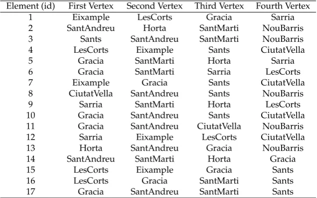
Table 1.Tetrahedral elements derived from the Delaunay Triangulation of the set of points.
Element (id) First Vertex Second Vertex Third Vertex Fourth Vertex
1 Eixample LesCorts Gracia Sarria
2 SantAndreu Horta SantMarti NouBarris
3 Sants SantAndreu SantMarti NouBarris
4 LesCorts Eixample Sants CiutatVella
5 Gracia SantMarti Horta Sarria
6 Gracia SantMarti Sarria LesCorts
7 Eixample Gracia Sants CiutatVella
8 CiutatVella SantAndreu Sants NouBarris
9 Sarria SantMarti Horta LesCorts
10 Gracia SantAndreu Sants CiutatVella
11 Gracia SantAndreu CiutatVella NouBarris
12 Sarria Eixample LesCorts CiutatVella
13 Horta SantAndreu Gracia NouBarris
14 SantAndreu SantMarti Horta Gracia
15 LesCorts Eixample Gracia Sants
16 LesCorts Gracia SantMarti Sants
17 Gracia SantAndreu SantMarti Sants
3. Results 193
In the present section, we demonstrate the application of this methodology to quantify the 194
temporal change of an urban multivariate system (see Figure 3). First, we cite the case study 195
that includes the multivariate description of the ten districts of Barcelona, and whose reduced 196
three-dimensional data-set is used as the starting point. Then, we derive the strain-rate state of 197
the data-set, pursuing the extension and contraction patterns visualization. Finally, we close this 198
section with insights about the city transformation implied in the strain-rate state of the data cloud. 199
3.1. Time-dependent data cloud from an urban multivariate description 200
The time-dependent data cloud comes from the PCA output of a multivariate description of the 201
city of Barcelona. Since 1987, the city has been divided into 10 administrative districts, which are the 202
largest territorial units of the city and can be compared with neighborhoods in a common metropolitan 203
area: Ciutat Vella, Eixample, Gràcia, Les Corts, Sarria, Sant Andreu, Sant Marti, Horta, Sants, and Nou 204
Barris. Barcelona has a population of approximately 1.6 million inhabitants living in 10216 ha. The 205
inclusion of all the 10 districts in the multivariate description has been aimed to represent the city at its 206
overall scale and to allow comparisons between them. 207
The raw multivariate description -from which the PCA is calculated- comprises the data of 40 208
environmental, economic, and social indicators for the ten districts in the time span oft0=2003≤ 209
tn ≤2015=tN,n=0, 1, .., 12. Hence, the case study data cloud comes from a PCA reduction of the 210
higher-dimensional multivariate data-setYn(tn)∈R40, into a lower-dimensional oneXn(tn)∈R3 211
that possesses only three independent dimensions: PC1, PC2, and PC3. The dimensionally-reduced 212
data-set from the application of the PCA is presented in AppendixA. Hence, the three-dimensional 213
and time-dependent data cloud is composed by the coordinatesXn(tn)of then=10 total number of
214
pointspidefined in the sequence ofN=12 time-steps from 2003 to 2015, with the time-step size of
215
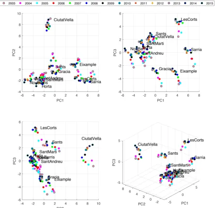
δt=1 year. These points are displayed in Figure2, where all the observations -districts each year- in 216
the time-span are included. 217
As the first step of our methodology, we apply the Delaunay Triangulation (DT) to the data 218
cloud. Specifically, we calculate the DT to the set of coordinates at each time-step Xn(tn). This
219
results in a meshTh(tn)composed bynel =|K|non-overlapping tetrahedron. Table1expands the
220
resulting triangulation for year 2003, with the vertices information for the nel = 17 tetrahedron. 221
Since the positionxi(tn)of a given pointpiat a later time-step can surpass the initial tetrahedron’s
222
Multivariate and time-dependent data-set Principal Component Analysis 3D and time-dependent data cloud Delaunay triangulation Finite Element
Interpolation Strain-Rate calculation
Eigenspace components
T
ime
statistics
Eigenspace statistics
Eigenspace components trajectories
Eigenspace components trajectories
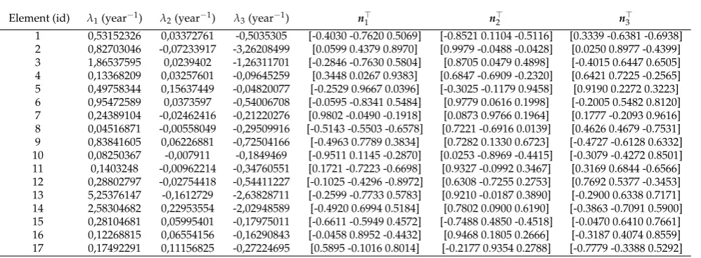
Table 2.Principal strain-rate components. Eigenvalues and Eigenvectors of the strain-rate tensor at the year 2003. The extension is denoted by the maximum eigenvalueλ1, and contraction is denoted by the
minimum eigenvalueλ3.
Element (id) λ1(year−1) λ2(year−1) λ3(year−1) n>1 n2> n>3
1 0,53152326 0,03372761 -0,5035305 [-0.4030 -0.7620 0.5069] [-0.8521 0.1104 -0.5116] [0.3339 -0.6381 -0.6938]
2 0,82703046 -0,07233917 -3,26208499 [0.0599 0.4379 0.8970] [0.9979 -0.0488 -0.0428] [0.0250 0.8977 -0.4399]
3 1,86537595 0,0239402 -1,26311701 [-0.2846 -0.7630 0.5804] [0.8705 0.0479 0.4898] [-0.4015 0.6447 0.6505]
4 0,13368209 0,03257601 -0,09645259 [0.3448 0.0267 0.9383] [0.6847 -0.6909 -0.2320] [0.6421 0.7225 -0.2565]
5 0,49758344 0,15637449 -0,04820077 [-0.2529 0.9667 0.0396] [-0.3025 -0.1179 0.9458] [0.9190 0.2272 0.3223]
6 0,95472589 0,0373597 -0,54006708 [-0.0595 -0.8341 0.5484] [0.9779 0.0616 0.1998] [-0.2005 0.5482 0.8120]
7 0,24389104 -0,02462416 -0,21220276 [0.9802 -0.0490 -0.1918] [0.0873 0.9766 0.1964] [0.1777 -0.2093 0.9616]
8 0,04516871 -0,00558049 -0,29509916 [-0.5143 -0.5503 -0.6578] [0.7221 -0.6916 0.0139] [0.4626 0.4679 -0.7531]
9 0,83841605 0,06226881 -0,72504166 [-0.4963 0.7789 0.3834] [0.7282 0.1330 0.6723] [-0.4727 -0.6128 0.6332]
10 0,08250367 -0,007911 -0,1849469 [-0.9511 0.1145 -0.2870] [0.0253 -0.8969 -0.4415] [-0.3079 -0.4272 0.8501]
11 0,1403248 -0,00962214 -0,34760551 [0.1721 -0.7223 -0.6698] [0.9327 -0.0992 0.3467] [0.3169 0.6844 -0.6566]
12 0,28802797 -0,02754418 -0,54411227 [-0.1025 -0.4296 -0.8972] [0.6308 -0.7255 0.2753] [0.7692 0.5377 -0.3453]
13 5,25376147 -0,1612729 -2,63828711 [-0.2599 -0.7733 0.5783] [0.9210 -0.0187 0.3890] [-0.2900 0.6338 0.7171]
14 2,58304682 0,22953554 -2,02948589 [-0.4920 0.6994 0.5184] [0.7802 0.0900 0.6190] [-0.3863 -0.7091 0.5900]
15 0,28104681 0,05995401 -0,17975011 [-0.6611 -0.5949 0.4572] [-0.7488 0.4850 -0.4518] [-0.0470 0.6410 0.7661]
16 0,12268815 0,06554156 -0,16290843 [-0.0458 0.8952 -0.4432] [0.9468 0.1805 0.2666] [-0.3187 0.4074 0.8559]
17 0,17492291 0,11156825 -0,27224695 [0.5895 -0.1016 0.8014] [-0.2177 0.9354 0.2788] [-0.7779 -0.3388 0.5292]
3.2. Principal strain-rates 224
We compute the strain-rate tensor of each tetrahedron with the interpolated version of the 225
velocities for the case study, such that linear piece-wise polynomial functions defined inside each 226
tetrahedron are used in the FEM interpolation. Certainly, we suppose that the velocities come from an 227
infinitesimal analysis in which the higher order terms of the displacement are neglected. The gradients 228
inside each tetrahedron are also considered to be constant since the polynomial functions are of first 229
order. Applying (10), we compute the strain-rate tensor of every tetrahedron,E(K,tn)for time-steps 230
n = 0, . . . , 11, since displacements cannot be calculated for the last yeart12 = 2015. Note that the 231
strain-rate tensor units are year−1(for the case study). 232
We are interested in the magnitude and orientations of the principal strain-rates -extension and 233
contraction- at the elemental level. Hence, the next step is to solve (12) and obtain the eigenspace 234
components (eigenvalues and eigenvectors) of the strain-rate tensor. For the sake of conciseness, we 235
list in Table2the results of the principal strain-rates for the year 2003 solely. 236
The application of this methodology to the case study is displayed graphically in Fig.3, beginning 237
with the map of the ten districts of Barcelona as the abstraction of the multivariate and time-dependent 238
dataset. The three-dimensional coordinates arising from the PCA output are displayed next. We 239
also present next the triangulated mesh at the initial year 2003, where kinematic depictions of the 240
point-wise displacements following (6) are plot as velocity vectors. It is clear from the visual inspection 241
that the quantitative analysis of the temporal transformation is greatly justified, so that we calculate 242
the strain-rate tensor over the FEM interpolation of discrete velocities and compute its principal 243
components. 244
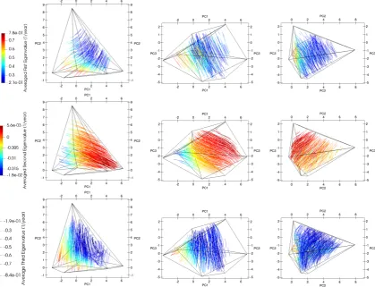
3.2.1. Trajectory patterns of the principal strain-rates 245
In favor of the analysis, we display the principal strain-rate components in a graphical way. 246
One first approach is to illustrate the patterns of extension-rate and contraction-rate using a vector 247
representation, to what is referred as theStrain-rate diagrams[21]. In that approach, the centroid of the 248
tetrahedron serves as the location from which the principal components of the strain-rate tensor give 249
a representative result inside the element. We draw the strain-rate diagram of the year 2003 in the 250
sixth step of Fig.3, where extension-rate is represented by symmetric blue vectorsλ1n1pointing out 251
visualize the distribution of the principal strain-rates and their three-dimensional orientations using 253
this type of illustration. 254
Our approach to ease the visualization and understanding of the strain-rate state is to draw 255
thetrajectoriesof the principal strain-rate components, as used for displaying stresses in beams and 256
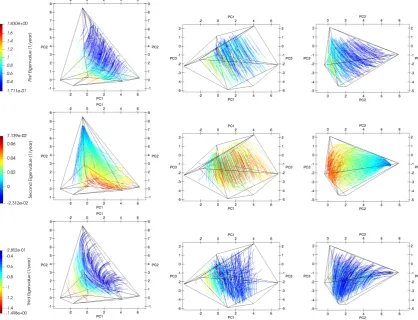
columns in [36]. In the following we demonstrate our findings of the strain-rate state at the year 257
2003 using the trajectories visualization. In Figure4we display the principal components trajectories, 258
where the lines are colored by the magnitude of the principal strain-rate and those are parallel to 259
its orientation. From these representations, we can understand the magnitude and orientation of 260
each principal component of the strain-rate tensor. And more importantly, the trajectory patterns 261
overlapped with the coordinates of the districts (in Figure2) provide information about local regions 262
of extension and contraction rates inside the urban description, where extension-rate patterns means 263
differentiation and contraction-rate patterns means clustering -or homogenization-. 264
In the case of the first strain-rate component which is shown at the top of Fig4, we observe that 265
the larger magnitude of extension-rate is localized in between Nou Barris Sant Andreu, Sant Marti, 266
Horta and Sants, and that it decreases near Eixample, Les Corts, and Ciutat Vella. Therefore, the main 267
transformation is located at the first cluster of districts: Nou Barris, Sant Andreu, Sant Marti, and 268
Horta. The extension-rate patterns are oriented from this cluster apart to Ciutat Vella, suggesting that 269
there is a divergence of Ciutat Vella from the clustered districts. Indeed, the main extension pattern 270
is oriented along the PC3 dimension and covers the clustered districts. It is of lesser importance the 271
pattern which comprises the districts of Nou Barris, Sant Marti, and Sants and ends at Gracia and 272
Eixample. 273
Contraction-rate, on the other hand, is expressed by the third principal strain-rate component, 274
which by definition is orthogonal to the first and second principal strain-rates. The third principal 275
strain-rate component is shown at the bottom of Fig.4, where we can appreciate this orthogonality by 276
noticing that the trajectories of the third principal strain-rate are perpendicular to the extension-rate 277
pattern. We observe that the contraction-rate trajectories are mostly homogeneous, with a minor 278
importance between Sant Marti, Sant Andreu, Nou Barris and Horta districts, and completely 279
declining at Sants and Gracia. This direct relation between extension and contraction is found in solids 280
deformations, where it is ruled by the conservation of mass -or Poisson ratio- [15]. 281
Apart from the extension and contraction patterns of the mesh, locations of smaller strain-rates 282
are represented by the second principal component. Considering the middle plots of Fig.4, we 283
recognize that the orientation of this strain-rate component is concentrated in between Les Corts, 284
Sarria, Horta and Nou Barris, and that it is directed towards Eixample, fading at Ciutat Vella. This 285
principal strain-rate component is certainly orthogonal to the first and second components, but it 286
implies a strain-rate pattern that is two orders of magnitude smaller. 287
In the previous lines we have demonstrated the application of the trajectories diagrams of the 288
principal strain-rate components as a powerful visualization technique of the three-dimensional 289
strain-rate state of a data cloud. The strain-rate patterns can be used to analyze the system’s 290
development, in example, with the identification of regions with a special behavior: although there are 291
some clustered districts in the case study, all of those are separating at a high rate in dimensions 1 and 292
3. Hence, those are differentiating themselves in the PC1 and PC3 description. On the contrary, low 293
strain-rates can be an indication of stagnation, and thus, an expression of inactivity where an abrupt 294
change is not probably to occur. That is specially the case of the Ciutat Vella district, which is separated 295
from the clustered nodes but it is neither diverging nor converging to them. 296
One final remark to the visualization of strain-rate patterns is that the principal strain-rate 297
trajectory plots are mesh independent: different triangulations will produce different positions, 298
magnitudes and orientations of the principal strain-rate components, nevertheless, trajectory lines 299
Table 3.Time-averaged eigenspace components.
Element(id) λ1(year−1) λ2(year−1) λ3(year−1) n>1 =⇒ λ1 n>2 =⇒ λ2 n>3 =⇒ λ3
1 0,1157 -0,0086 -0,0687 [-0.4941 -0.4365 0.7519] [0.1770 0.1339 -0.9751] [0.1682 0.8390 0.5175]
2 0,5087 -0,0085 -0,8859 [-0.5777 0.5570 0.5966] [-0.4259 -0.1592 -0.8907] [-0.0636 -0.9309 0.3596]
3 0,3919 -0,0440 -0,1662 [-0.3746 -0.7054 0.6017] [-0.9963 0.0335 0.0789] [0.3127 -0.7926 -0.5234]
4 0,0868 0,0041 -0,0193 [0.4684 0.8217 0.3247] [-0.0619 0.3756 -0.9247] [-0.7437 -0.4144 -0.5246]
5 0,0435 -0,0326 -0,0659 [-0.2319 0.8799 0.4148] [-0.0891 -0.1728 0.9809] [0.2229 -0.2816 -0.9333]
6 0,1834 0,0096 -0,0536 [-0.2271 -0.8440 0.4859] [-0.6281 0.2260 -0.7446] [-0.4216 0.8544 0.3038]
7 0,0647 -0,0059 -0,0485 [0.5157 -0.6416 0.5678] [0.0741 -0.9932 0.0893] [0.2985 -0.4332 -0.8504]
8 0,1436 -0,0198 -0,0174 [-0.3994 -0.4110 0.8194] [-0.1094 0.9614 -0.2525] [0.3984 -0.8684 -0.2952]
9 0,6311 0,0178 -0,1144 [-0.2472 -0.6917 0.6785] [0.2277 0.2955 0.9278] [0.1771 0.8523 0.4921]
10 0,0355 0,0098 -0,0745 [0.4275 0.8923 -0.1449] [0.8566 -0.5130 -0.0551] [-0.5198 0.2220 -0.8249]
11 0,0452 -0,0239 -0,1039 [0.4742 -0.0948 0.8753] [-0.7018 -0.6930 0.1650] [-0.3132 -0.9345 -0.1693]
12 0,2054 0,0336 -0,0703 [-0.5086 -0.8385 -0.1954] [0.1867 0.6566 0.7307] [0.0460 -0.4726 -0.8801]
13 1,1642 -0,0218 -0,3192 [-0.4080 -0.6299 0.6609] [-0.9632 0.2605 0.0654] [-0.5136 0.5798 -0.6325]
14 0,1923 0,0415 -0,2640 [-0.4758 0.8168 0.3264] [0.9570 0.2693 -0.1076] [0.4308 -0.2715 -0.8606]
15 0,0552 0,0085 -0,0363 [-0.2364 0.6160 0.7514] [0.7518 0.2783 -0.5978] [0.6817 0.6544 -0.3270]
16 0,0438 0,0175 -0,0059 [0.2794 0.9257 -0.2549] [0.8449 -0.2441 0.4760] [-0.5430 -0.2892 -0.7883]
17 0,2113 -0,0196 -0,3129 [-0.0062 0.9656 0.2599] [0.0760 0.2441 0.9668] [0.0666 -0.9959 -0.0609]
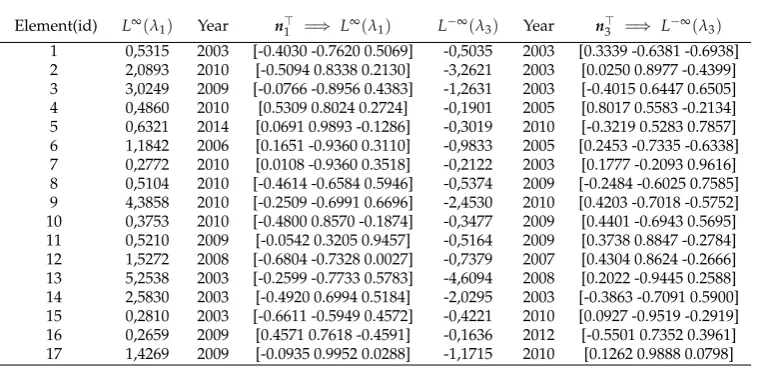
Table 4.Maximum and minimum eigenspace components in the time span.
Element(id) L∞(λ1) Year n>1 =⇒ L∞(λ1) L−∞(λ3) Year n3> =⇒ L−∞(λ3)
1 0,5315 2003 [-0.4030 -0.7620 0.5069] -0,5035 2003 [0.3339 -0.6381 -0.6938]
2 2,0893 2010 [-0.5094 0.8338 0.2130] -3,2621 2003 [0.0250 0.8977 -0.4399]
3 3,0249 2009 [-0.0766 -0.8956 0.4383] -1,2631 2003 [-0.4015 0.6447 0.6505]
4 0,4860 2010 [0.5309 0.8024 0.2724] -0,1901 2005 [0.8017 0.5583 -0.2134]
5 0,6321 2014 [0.0691 0.9893 -0.1286] -0,3019 2010 [-0.3219 0.5283 0.7857]
6 1,1842 2006 [0.1651 -0.9360 0.3110] -0,9833 2005 [0.2453 -0.7335 -0.6338]
7 0,2772 2010 [0.0108 -0.9360 0.3518] -0,2122 2003 [0.1777 -0.2093 0.9616]
8 0,5104 2010 [-0.4614 -0.6584 0.5946] -0,5374 2009 [-0.2484 -0.6025 0.7585]
9 4,3858 2010 [-0.2509 -0.6991 0.6696] -2,4530 2010 [0.4203 -0.7018 -0.5752]
10 0,3753 2010 [-0.4800 0.8570 -0.1874] -0,3477 2009 [0.4401 -0.6943 0.5695]
11 0,5210 2009 [-0.0542 0.3205 0.9457] -0,5164 2009 [0.3738 0.8847 -0.2784]
12 1,5272 2008 [-0.6804 -0.7328 0.0027] -0,7379 2007 [0.4304 0.8624 -0.2666]
13 5,2538 2003 [-0.2599 -0.7733 0.5783] -4,6094 2008 [0.2022 -0.9445 0.2588]
14 2,5830 2003 [-0.4920 0.6994 0.5184] -2,0295 2003 [-0.3863 -0.7091 0.5900]
15 0,2810 2003 [-0.6611 -0.5949 0.4572] -0,4221 2010 [0.0927 -0.9519 -0.2919]
16 0,2659 2009 [0.4571 0.7618 -0.4591] -0,1636 2012 [-0.5501 0.7352 0.3961]
3.3. Temporal statistics of the principal strain-rates 301
Plots of the principal strain-rate components trajectories can be completed for the remaining years 302
of the time span,tn,n= 1, 2, ..., 11, and those are attached as meta-data in the electronic version of
303
the present article. Readings of the strain-rate streamline patterns for those years can be completed 304
straightforwardly as discussed in the paragraphs above. Nevertheless, we perform some temporal 305
statistics of the strain-rate states, where the principal strain-rates calculated for each time-step are 306
accounted as the temporal events: each strain-rate state is accounted as a single observation. 307
The first statistics that we perform is the time-average of the principal strain-rate components, 308
separated as the first, second, and third principal strain-rates. Table3presents the time-averaged 309
results of the principal strain-rates. Also, in the last schematic of Fig.3, we plot the strain-rate diagram 310
of the time-averaged principal strain-rates at the time-averaged centroid of tetrahedron elements. This 311
figure gives insights about the orientation and magnitude of the first and third principal strain-rates, 312
again by plotting the symmetric arrows pointing out for extension and pointing in for contraction. We 313
complete our analysis by drawing the trajectory curves of those time-averaged strain-rate diagrams in 314
Fig.5. 315
With the aid of Figures2and5we analyze the trajectory patterns of the time-averaged strain-rate 316
state of the data cloud. In the case of the first and third strain-rate components, those are comparable 317
to the ones described in the previous paragraphs for the year 2003. We observe a high extension-rate 318
behavior between Nou Barris, Sant Andreu and Horta in the PC1 dimension. The contraction-rate, 319
on the other side, is oriented in the PC2 dimension and it is mostly located in between Gracia and 320
Eixample and decreases near Sants. In the case of the contraction-rate in the PC3 dimension, it is 321
mostly present between Nou Barris and Horta, and in smaller magnitude between Horta and Sant 322
Andreu. The contraction-rate between the remaining districts is negligible in all dimensions. Both the 323
extension and contraction rates demonstrate trajectory patterns which are directed from the clustered 324
districts towards the separated district of Ciutat Vella. However, the magnitude of the time-averaged 325
strain-rates is much smaller than the ones obtained for year 2003. In the case of the time-averaged 326
second strain-rate, its magnitude is greater for Eixample, Les Corts, and Sarria nodes than for the 327
clustered nodes. The orientation of the trajectories involving this second strain-rate component is 328
parallel to the one linking Eixample and Les Corts to the clustered nodes. 329
The second temporal statistics that we perform is to calculateL∞−norm of the temporal strain-rate 330
distribution. That is, to calculate the year where the maximum extension and contraction rates occur 331
within each tetrahedron. The results of the application of theL∞−norm to the case study are presented 332
in Table4. We observe that the maximum strain-rates occur at year 2003: either expansion or contraction. 333
Also, that important contraction-rate magnitudes take place between the years 2003 and 2010. This is 334
not the case of the extension-rate magnitudes, which are more prevalent after year 2008. 335
4. Conclusions 336
In the present article, we have quantified the temporal change of a time-dependent and 337
three-dimensional dataset. Contrary to other approaches [1], we have calculated the three-dimensional 338
strain-rate state of the dataset based on the interpolation of discrete point-wise displacements -or 339
data variations-. We have applied a technique in continuum mechanics using a FEM interpolation of 340
non-overlapping linear tetrahedral elements that spans the three-dimensional dataset. 341
The methodology has demonstrated to exhibit regions of major deformation-rate. Departing from 342
the calculation of the numerical strain-rate values, we have introduced some data-visualization 343
techniques that help to locate the magnitudes and orientations of the strain-rate state in the 344
three-dimensional framework. This is the case of the principal strain-rate trajectories, whose have 345
demonstrated to be more detailed than other possible visualization techniques, e.g. strain-rate diagrams 346
in [24,28]. The main difference with strain-rate diagrams is the ability of the former to visualize a 347
continuum version of the strain-rate inside the dataset, and to separate the analysis into each principal 348
The calculation of the strain-rate state shows that the methodology is suitable for quantifying 350
the temporal change of a reduced three-dimensional dataset describing the social, economic and 351
environmental state of the city of Barcelona. In particular, high strain-rates are associated with the 352
localized deformation of regions that represent the districts of the city in the time span of 13 years. It is 353
similar toCluster Analysis[37–39] orDistance measures[40], in the sense that the method portrays the 354
similarities and differences between the districts of the city. The distinctive attribute of the present 355
work is the feasibility to quantify the districts’ differentiation with time: the strain-rate tensor provides 356
quantitative information about local regions of extension and contraction, where extension-rate patterns 357
means differentiation and contraction-rate patterns means clustering -or homogenization-. Conclusions 358
about the divergence or clustering of districts in time can therefore be stated. For example, it reveals 359
the time, location, and orientation of pressures affecting the inhabitants of certain districts of the city, 360
essentially those which are rapidly diverging from the rest (e.g. the case of Ciutat Vella for the case 361
study). This methodology locates regions where detailed action is necessary, as well as the foretelling 362
of possible ruptures in the system. 363
Finally, we would like to say that this method is not limited to the study of the data change, 364
but can also be applied to other descriptions: a natural sequel to the present article is the study of 365
the time-dependent data cloud as a deforming elastic solid under equilibrium. Solving the inverse 366
problem, namely the identification of the constitutive moduli of the deforming material emerges as the 367
first step for predicting the system’s future state given its historical data. 368
Author Contributions:The authors equally contributed to the elaboration of this article.
369
Funding:This research received no external funding.
370
Acknowledgments:Lorena Salazar-Llano greatly acknowledges the financial support received by the pre-doctoral
371
grant “Beca Rodolfo Llinás para la promoción de la formación avanzada y el espíritu científico de Bogotá” from
372
Fundación CEIBA.
373
Conflicts of Interest:The authors declare no conflict of interest.
374
Appendix A 375
References 376
1. Fuchs, R.; Hauser, H. Visualization of multi-variate scientific data. Computer Graphics Forum. Wiley
377
Online Library, 2009, Vol. 28, pp. 1670–1690.
378
2. Salazar-Llano, L.; Rosas-Casals, M.; Ortego, M.I. An Exploratory Multivariate Statistical Analysis to Assess
379
Urban Diversity. SustainabilitySubmitted.
380
3. White, F.M.; Corfield, I.Viscous fluid flow; Vol. 3, McGraw-Hill New York, 2006.
381
4. Bower, A.F.Applied mechanics of solids; CRC press, 2009.
382
5. McLoughlin, T.; Laramee, R.S.; Peikert, R.; Post, F.H.; Chen, M. Over two decades of integration-based,
383
geometric flow visualization. Computer Graphics Forum. Wiley Online Library, 2010, Vol. 29, pp.
384
1807–1829.
385
6. Süßmuth, J.; Winter, M.; Greiner, G. Reconstructing animated meshes from time-varying point clouds.
386
Computer Graphics Forum. Wiley Online Library, 2008, Vol. 27, pp. 1469–1476.
387
7. Ustinin, M.N.; Kronberg, E.; Filippov, S.V.; Sytchev, V.V.; Sobolev, E.V.; Llinás, R. Kinematic visualization of
388
human magnetic encephalography. 2010,5, 176–187.
389
8. Wang, S.W.; Interrante, V.; Longmire, E. Multivariate visualization of 3D turbulent flow data. Visualization
390
and Data Analysis 2010. International Society for Optics and Photonics, 2010, Vol. 7530, p. 75300N.
391
9. Kohler, M.; Krzy ˙zak, A. Nonparametric estimation of non-stationary velocity fields from 3D particle
392
tracking velocimetry data. Computational Statistics & Data Analysis2012,56, 1566–1580.
393
10. Aguirre-Pablo, A.; Aljedaani, A.B.; Xiong, J.; Idoughi, R.; Heidrich, W.; Thoroddsen, S.T. Single-camera 3D
394
PTV using particle intensities and structured light.Experiments in Fluids2019,60, 25.
395
11. Keim, D.A. Information visualization and visual data mining. IEEE transactions on Visualization and 396
Computer Graphics2002,8, 1–8.
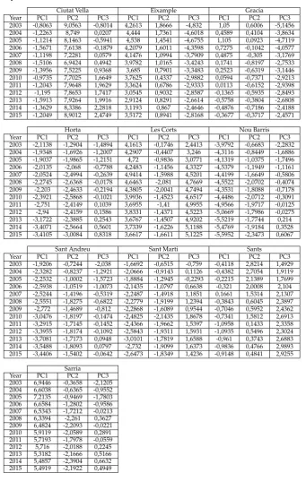
Table A1.Coordinates (seen as the component loadings of the PCA analysis) for the ten districts in the temporal span.
Ciutat Vella Eixample Gracia
Year PC1 PC2 PC3 PC1 PC2 PC3 PC1 PC2 PC3
2003 -0,8063 9,0563 -0,8014 4,2613 1,8666 -4,832 1,05 0,6006 -5,1456 2004 -1,2263 8,749 0,0207 4,444 1,7361 -4,6018 0,4589 0,4104 -3,8634 2005 -1,1214 8,1463 -0,5941 4,538 1,4541 -4,6755 1,105 0,0923 -4,7119 2006 -1,5671 7,6138 -0,1879 4,2079 1,6011 -4,3598 0,7275 -0,1042 -4,0577 2007 -1,1198 7,2281 0,0579 4,1476 1,0994 -3,7909 0,4875 -0,305 -3,1769 2008 -1,5106 6,9424 0,4942 3,9782 1,0165 -3,4243 0,1741 -0,8197 -2,7533 2009 -1,3956 7,5225 0,9368 3,685 0,7901 -3,3483 0,2523 -0,6319 -3,1446 2010 -0,9735 7,7025 1,6649 3,7625 0,4337 -2,9882 0,0594 -0,7371 -2,9213 2011 -1,2043 7,9648 1,9629 3,3624 0,6786 -2,9333 0,0113 -0,6152 -2,9398 2012 -1,195 7,8653 1,7417 3,0545 0,9032 -2,8587 -0,1365 -0,5935 -2,8493 2013 -1,5913 7,9264 1,9916 2,9124 0,8291 -2,6614 -0,5758 -0,3804 -2,6808 2014 -1,3629 8,3386 2,2818 3,1193 0,867 -2,4646 -0,4876 -0,7186 -2,4188 2015 -1,2049 8,9012 2,4749 3,5172 0,8941 -2,8168 -0,3677 -0,3717 -2,4571
Horta Les Corts Nou Barris
Year PC1 PC2 PC3 PC1 PC2 PC3 PC1 PC2 PC3
2003 -2,1138 -1,2904 -1,4894 4,1613 -0,1746 2,4413 -3,9792 -0,6683 -2,2832 2004 -1,9348 -1,6926 -1,2007 4,2907 -0,4407 3,246 -4,3116 -0,8449 -1,6886 2005 -1,9037 -1,9865 -1,2151 4,72 -0,9836 3,0771 -4,1319 -1,0375 -1,7496 2006 -2,0135 -2,068 -0,7788 4,2483 -1,1456 4,3327 -4,5379 -1,1949 -1,1161 2007 -2,0524 -2,4994 -0,2639 4,9414 -1,5988 4,5201 -4,4199 -1,6649 -0,5806 2008 -2,2745 -2,6368 -0,0178 4,6463 -2,081 4,7669 -4,5522 -2,0702 -0,4074 2009 -2,203 -2,4633 -0,2194 4,3805 -2,0041 4,7494 -4,3531 -1,8088 -0,7178 2010 -2,3921 -2,5868 -0,1021 3,9936 -1,4523 4,6517 -4,4486 -2,0712 -0,3091 2011 -2,751 -2,4149 0,1039 3,6955 -1,41 4,9955 -4,9566 -1,9717 -0,0125 2012 -2,94 -2,4159 0,1586 3,8331 -1,4371 4,5223 -5,0669 -1,7986 -0,0275 2013 -3,1722 -2,3885 0,2543 3,6767 -1,4507 4,9202 -5,5219 -1,7744 0,214 2014 -3,4071 -2,5664 0,5601 3,7339 -1,6226 5,1188 -5,4769 -1,9184 0,3528 2015 -3,4105 -3,0084 0,8318 3,6617 -1,6611 5,1225 -5,5952 -2,3473 0,6067
Sant Andreu Sant Marti Sants
Year PC1 PC2 PC3 PC1 PC2 PC3 PC1 PC2 PC3
2003 -1,9206 -0,7244 -2,038 -1,6692 -0,6515 -0,759 -0,4118 2,8214 1,4929 2004 -2,3282 -0,8237 -1,2921 -2,0666 -0,9143 0,1126 -0,4382 2,7054 1,9119 2005 -2,2532 -1,0002 -1,5723 -1,8884 -1,2945 -0,2293 -0,2215 2,1389 1,7699 2006 -2,5938 -1,0519 -1,0073 -2,1435 -1,0797 0,6638 -0,321 2,0008 2,104 2007 -2,5244 -1,4196 -0,5319 -2,2487 -1,4918 1,1851 0,1661 1,5314 2,1307 2008 -2,5551 -1,8275 -0,6822 -2,2779 -1,9199 1,2394 -0,3843 0,6045 2,3897 2009 -2,772 -1,4689 -0,812 -2,2868 -1,6089 0,9544 -0,7046 0,5952 2,4362 2010 -3,0476 -1,8197 -0,1474 -2,4825 -2,1435 1,8678 -0,7341 1,5812 2,6913 2011 -3,2915 -1,7145 -0,1452 -2,4366 -1,9662 1,5397 -1,0958 0,1433 2,3358 2012 -3,3955 -1,8174 -0,1092 -2,5843 -1,9311 1,5931 -1,0935 0,5496 2,3024 2013 -3,7081 -1,7173 0,0948 -3,0101 -1,7819 1,6588 -0,961 0,3743 2,6883 2014 -3,5488 -1,8093 0,0797 -2,732 -1,9099 1,6373 -0,9836 0,4766 2,9893 2015 -3,4406 -1,5402 -0,0642 -2,6473 -1,8349 1,4236 -0,9148 0,4841 2,9255
Sarria
Year PC1 PC2 PC3
12. Gao, L.; Heath, D.G.; Kuszyk, B.S.; Fishman, E.K. Automatic liver segmentation technique for
398
three-dimensional visualization of CT data.Radiology1996,201, 359–364.
399
13. Teplan, M.; others. Fundamentals of EEG measurement.Measurement science review2002,2, 1–11.
400
14. Wang, C.; Yu, H.; Ma, K.L. Importance-driven time-varying data visualization. IEEE Transactions on 401
Visualization and Computer Graphics2008,14, 1547–1554.
402
15. Mase, G.T.; Smelser, R.E.; Mase, G.E.Continuum mechanics for engineers; CRC press, 2009.
403
16. Marsden, J.E.; Hughes, T.J.Mathematical foundations of elasticity; Courier Corporation, 1994.
404
17. Xu, P.; Grafarend, E. Statistics and geometry of the eigenspectra of three-dimensional second-rank
405
symmetric random tensors. Geophysical Journal International1996,127, 744–756.
406
18. Wdowinski, S.; Sudman, Y.; Bock, Y. Geodetic detection of active faults in S. California. Geophysical research 407
letters2001,28, 2321–2324.
408
19. Straub, C.; Kahle, H.G.; Schindler, C. GPS and geologic estimates of the tectonic activity in the Marmara
409
Sea region, NW Anatolia. Journal of Geophysical Research: Solid Earth1997,102, 27587–27601.
410
20. Moin, P.Fundamentals of engineering numerical analysis; Cambridge University Press, 2010.
411
21. Hackl, M.; Malservisi, R.; Wdowinski, S. Strain rate patterns from dense GPS networks. Natural Hazards 412
and Earth System Sciences2009,9, 1177–1187.
413
22. Wang, H.; Amini, A.A. Cardiac motion and deformation recovery from MRI: A review. IEEE Transactions 414
on Medical Imaging2012,31, 487–503.
415
23. Pedrizzetti, G.; Sengupta, S.; Caracciolo, G.; Park, C.S.; Amaki, M.; Goliasch, G.; Narula, J.; Sengupta,
416
P.P. Three-dimensional principal strain analysis for characterizing subclinical changes in left ventricular
417
function. Journal of the American Society of Echocardiography2014,27, 1041–1050.
418
24. Cai, J.; Grafarend, E.W. Statistical analysis of geodetic deformation (strain rate) derived from the space
419
geodetic measurements of BIFROST Project in Fennoscandia. Journal of Geodynamics2007,43, 214–238.
420
25. Cai, J.; Grafarend, E.W. Statistical analysis of the eigenspace components of the two-dimensional, symmetric
421
rank-two strain rate tensor derived from the space geodetic measurements (ITRF92-ITRF2000 data sets) in
422
central Mediterranean and Western Europe. Geophysical Journal International2007,168, 449–472.
423
26. Mastrolembo, B.; Caporali, A. Stress and strain-rate fields: A comparative analysis for the Italian territory.
424
Bollettino di Geofisica Teorica ed Applicata2017,58.
425
27. Houlie, N.; Woessner, J.; Giardini, D.; Rothacher, M. Lithosphere strain rate and stress field orientations
426
near the Alpine arc in Switzerland. Scientific reports2018,8.
427
28. Su, X.; Yao, L.; Wu, W.; Meng, G.; Su, L.; Xiong, R.; Hong, S. Crustal deformation on the northeastern
428
margin of the Tibetan plateau from continuous GPS observations. Remote Sensing2019,11, 34.
429
29. Sneddon, I.N. The distribution of stress in the neighbourhood of a crack in an elastic solid. Proceedings of 430
the Royal Society of London. Series A. Mathematical and Physical Sciences1946,187, 229–260.
431
30. Williams, M. The bending stress distribution at the base of a stationary crack. Trans. ASME1957,
432
79, 109–114.
433
31. Aktu ˘g, B.; Parmaksız, E.; Kurt, M.; Lenk, O.; Kılıço ˘glu, A.; Gürdal, M.A.; Özdemir, S. Deformation of
434
central anatolia: GPS implications.Journal of Geodynamics2013,67, 78–96.
435
32. Grafarend, E. Criterion matrices for deforming networks. InOptimization and design of geodetic networks;
436
Springer, 1985; pp. 363–428.
437
33. Grafarend, E.W. Three-dimensional deformation analysis: Global vector spherical harmonic and local
438
finite element representation.Tectonophysics1986,130, 337–359.
439
34. Dermanis, A.; Grafarend, E. The finite element approach to the geodetic computation of two-and
440
three-dimensional deformation parameters: A study of frame invariance and parameter estimability.
441
International Conference “Cartography-Geodesy”, Maracaibo, Venezuela, 1992.
442
35. Marot, C.; Pellerin, J.; Remacle, J.F. One machine, one minute, three billion tetrahedra.International Journal 443
for Numerical Methods in Engineering,0,[https://onlinelibrary.wiley.com/doi/pdf/10.1002/nme.5987].
444
doi:10.1002/nme.5987.
445
36. Gere, J.M.; Goodno, B.J. Mechanics of Materials, Brief Edition. Cengage Learning2012.
446
37. Clemants, S.; Moore, G. Patterns of species diversity in eight northeastern United States cities. Urban 447
habitats2003,1.
448
38. Raudsepp-Hearne, C.; Peterson, G.D.; Bennett, E.M. Ecosystem service bundles for analyzing tradeoffs in
449
diverse landscapes.Proceedings of the National Academy of Sciences2010,107, 5242–5247.
39. Dossa, L.H.; Abdulkadir, A.; Amadou, H.; Sangare, S.; Schlecht, E. Exploring the diversity of urban and
451
peri-urban agricultural systems in Sudano-Sahelian West Africa: An attempt towards a regional typology.
452
Landscape and urban planning2011,102, 197–206.
453
40. Laliberté, E.; Legendre, P. A distance-based framework for measuring functional diversity from multiple
454
traits.Ecology2010,91, 299–305.