Modification of the Riemann problem and the application for the boundary conditions in computational fluid dynamics

(1)

Modiﬁcation of the Riemann problem and the application for the boundary

conditions in computational ﬂuid dynamics

MartinKyncl1,a_and_Jaroslav_Pelant1,b

1_{Aerospace Research and Test Establishment (VZL ´}_U),

Beranov´ych 130, 199 05 Praha - Letˇnany, Czech Republic

Abstract. We work with the system of partial differential equations describing the non-stationary compressible turbulent fluid flow. It is a characteristic feature of the hyperbolic equations, that there is a possible raise of discontinuities in solutions, even in the case when the initial conditions are smooth. The fundamental problem in this area is the solution of the so-called Riemann problem for the split Euler equations. It is the elementary problem of the one-dimensional conservation laws with the given initial conditions (LIC - left-hand side, and RIC - right-hand side). The solution of this problem is required in many numerical methods dealing with the 2D/3D fluid flow. The exact (entropy weak) solution of this hyperbolical problem cannot be expressed in a closed form, and has to be computed by an iterative process (to given accuracy), therefore various approximations of this solution are being used. The complicated Riemann problem has to be further modified at the close vicinity of boundary, where the LIC is given, while the RIC is not known. Usually, this boundary problem is being linearized, or roughly approximated. The inaccuracies implied by these simplifications may be small, but these have a huge impact on the solution in the whole studied area, especially for the non-stationary flow. Using the thorough analysis of the Riemann problem we show, that the RIC for the local problem can be partially replaced by the suitable complementary conditions. We suggest such complementary conditions accordingly to the desired preference. This way it is possible to construct the boundary conditions by the preference of total values, by preference of pressure, velocity, mass flow, temperature. Further, using the suitable complementary conditions, it is possible to simulate the flow in the vicinity of the diffusible barrier. On the contrary to the initial-value Riemann problem, the solution of such modified problems can be written in the closed form for some cases. Moreover, using such construction, the local conservation laws are not violated. Algorithms for the solution of the modified Riemann problems were coded and used within our own developed code for the solution of the compressible gas flow (the Euler, the Navier-Stokes, and the RANS equations). Numerical examples show superior behaviour of the suggested boundary conditions. Constructed boundary conditions are robust and accelerate the convergence of the method. The original result of our work is the analysis of various modifications of the Riemann problem and its applications.

1 Introduction

Undoubtedly, the boundary conditions play important role in the computational fluid dynamics (CFD). We work with the system of equations describing non-stationary compress-ible turbulent fluid flow, i.e. the Reynolds-Averaged Navier-Stokes (RANS) equations in 2D and 3D. We focus on the numerical solution of these equations, and on the bound-ary conditions. We suggest the original approach to the boundary conditions. The aim is to satisfy the conserva-tion laws in the close vicinity of the boundary. Usually, the boundary problem is being linearized, or roughly aprox-imated. The inaccuracies implied by these simplifications may be small, but it has a huge impact on the solution in the whole studied area, especially for the non-stationary flow. In our approach we try to be as exact as possible. There-fore we use the analysis of the so-called Riemann problem

for the 2D/3D split Euler equations in order to construct

the boundary values (for the density, velocity, pressure).

a _e-mail:_{[email protected]} b _e-mail:_{[email protected]}

We solve the boundary modiﬁcations of this initial-value problem. The crucial problem of many numerical methods for the solution of the compressible ﬂow lies in the

evalu-ation of the so-called ﬂuxes through the edges/facesΓi jof

the particular elements. The state values in the vicinity of

the edgeΓi jare known at time instanttk, and these values

form the initial conditions (LIC - left-hand side, and RIC - right-hand side) for the so-called Riemann problem for

the 2D/3D split Euler equations. The exact (entropy weak)

(2)

[13, pages 221-225], where the RIC is constructed in a spe-cial way, in order to obtain the desired solution. Using the analysis of the Riemann problem we show, that the RIC for the local problem can be partially replaced by the suitable complementary condition. Some of the suggested bound-ary conditions were shown in [8] (by preference of pres-sure, temperature, velocity,...). We complement the bound-ary problem suitably, and we show the analysis of the re-sulting uniquely-solvable modiﬁed Riemann problem. We construct own algorithm for the solution of this boundary problem. It can be used within various methods in CFD. The algorithm was coded and used within our own devel-oped code for the solution of the compressible gas ﬂow (the Euler, NS, and RANS equations).

2 The Riemann Problem for the Split Euler

Equations

For many numerical methods dealing with the two or three dimensional equations, describing the compressible ﬂow,

it is useful to solve the Riemann problem for the3D split

Euler equations. We search the solution of the system of

partial diﬀerential equations in timetand space (x, y,z)

∂ ∂t +

∂u

∂x =0

∂u

∂t +

∂(p+u2₎

∂x =0

∂v ∂t +

∂uv

∂x =0

∂w ∂t +

∂uw ∂x =0

∂E

∂t +

∂u(E+p) ∂x =0,

(1)

equipped with the initial conditions

(x,t)=L,u(x,t)=uL,p(x,t)=pL, x<0, (2)

(x,t)=R,u(x,t)=uR,p(x,t)=pR, x>0. (3)

Vectoru=(u, v, w) denotes the velocity,density,p

pres-sure,E=e+|u|2_{is the total energy, with}_e_{denoting the}

speciﬁc internal energy. We assume the equation of state for the calorically ideal gas

e= p

(γ−1).

‘Split’ means here that we still have 5 equations in 3D,

but the dependence ony,z(space coordinates) is neglected,

and we deal with the system for one space variablex. The

system (1) is considered in the setQ_∞=(−∞,∞)×(0,+∞).

The solution of this problem is fundamentally the same as the solution of the Riemann problem for the 1D Eu-ler equations, see [9, page 138]. In fact, the solution for the pressure, the ﬁrst component of the velocity, and the density is exactly the same as in one-dimensional case. It is a characteristic feature of the hyperbolic equations, that there is a possible raise of discontinuities in solutions, even in the case when the initial conditions are smooth, see [12, page 390]. Here the concept of the classical solution is too restrictive, and therefore we seek a weak solution of this problem. To distinguish physically admissible so-lutions from nonphysical ones, entropy condition must be introduced, see [12, page 396]. By the solution of the

prob-lem (1),(2),(3) we mean theweak entropy solutionof this

problem inQ_∞. The analysis to the solution of this

prob-lem can be found in many books, i.e. [9], [12], [13]. The

general theorem on the solvability of the Riemann problem can be found in [9, page 88].

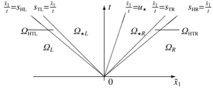
The solution is piecewisesmoothand its general form

can be seen in Fig. 1, where the system of half lines is drawn.

-6t

˜

x1

0

@ @ @ @ @ @

l l l l l l l l

,,

˜ x1

t=sHL sTL=

˜ x1

t

˜ x1

t=u ˜ x1

t=sTR sHR=

˜ x1

t

ΩHTL

ΩL

ΩL ΩR

ΩR

ΩHTR

Fig. 1. Structure of the solution of the Riemann problem (1),(2),(3)

These half lines deﬁne regions, where solution is either constant or given by a smooth function. Let us deﬁne the

open sets calledwedges(see Fig. 1):

ΩL=wedge(L−∞,sHL),

ΩHTL=wedge(sHL,sTL),

ΩL=wedge(sTL,u∗),

ΩR =wedge(u,sTR),

ΩHTR=wedge(sTR,sHR),

ΩR =wedge(sHR,L+∞).

Using the theory in [9], [12], [13], we can write the solu-tion for the primitive variables as

(,u, v, w,p)|ΩL =(L,uL, vL, wL,pL),

(,u, v, w,p)|_ΩL =(L,u, vL, wL,p),

(,u, v, w,p)|_Ω_R =(R,u, vR, wR,p),

(,u, v, w,p)|ΩR =(R,uR, vR, wR,pR).

The folowing relations for these variables hold:

u=uL+

⎧⎪⎪ ⎪⎪⎪⎨ ⎪⎪⎪⎪⎪ ⎩

−(p−pL)

₂

(γ+1)L

p+γγ−+11pL

1

2

,p>pL

2 γ−1aL

1− p

pL

(γ−1)/2γ

,p≤pL

(4)

L=

⎧⎪⎪⎪ ⎪⎨

⎪⎪⎪⎪⎩L

γ−1 γ+1pLp+1

pL p+γ−

1 γ+1

,p>pL

L p_p_L

1

γ_, _p

≤pL

(5)

s1

T L=

⎧⎪⎪⎪ ⎨

⎪⎪⎪⎩uL−aL

γ+1 2γ

p pL +

γ−1

2γ, p>pL

u−aL p_p_L

(γ−1)/2γ

, p≤pL

(6)

u=uR+

⎧⎪⎪⎪ ⎪⎪⎨ ⎪⎪⎪⎪⎪ ⎩

(p−pR)

₂

(γ+1)R

p+γγ−+11pR

1

2

,p>pR,

− 2 γ−1aR

1− p_p_R(γ−1)/2γ

,p≤pR

(7)

R=

⎧⎪⎪⎪ ⎪⎨

⎪⎪⎪⎪⎩R

p pR+γ−

1 γ+1 γ−1 γ+1

p pR+1,

p>pR

R ppR

1

γ_, _p

≤pR

(8)

s3_{T R} =⎧⎪⎪⎪⎨_⎪⎪⎪⎩uR+aR

γ+1 2γ

p pR +

γ−1

2γ ,p>pR

u+aR p_p_R

(γ−1)/2γ

, p≤pR

(3)

HereaL =

γpL/L, aR =

γpR/R, andγdenotes

the adiabatic constant. Furthers1

T Ldenotes ”unknown left

wave speed”,s3

T R”unknown right wave speed”. Note, that

the system (4) - (9) is the system of 6 equations for 6

un-knownsp,u,LR,s1_{T L},s3_{T R}.

Solution for the Pressurep

The combination of the equations (4), (7) gives the implicit

equation for the unknown pressurep

uL+F1L(p)=uR+F3R(p),

with

F1L(p)=

⎧⎪⎪ ⎪⎪⎪⎨ ⎪⎪⎪⎪⎪ ⎩

−(p−pL)

₂

(γ+1)L

p+γ−1 γ+1pL

1 2

, p>pL

2

γ−1aL

1− _pp_L(γ−1)/2γ

, p≤pL.

,

F3R(p)=

⎧⎪⎪ ⎪⎪⎪⎨ ⎪⎪⎪⎪⎪ ⎩

(p−pR)

2

(γ+1)R

p+γ−1 γ+1pR

1 2

, p>pR,

− 2

γ−1aR

1− _pp

R (γ−1)/2γ

, p≤pR.

This is a nonlinear algebraic equation, and one cannot express the analytical solution of this problem in a closed

form. The solutionpcan be found as the root of the

func-tionF(p) deﬁned as

F(p)=F3R(p)−F1L(p)+uR−uL. (10)

The analysis of this function can be found in [9]. Here we

state, thatF(p) is monotone and concave. Also the analytic

expression for its derivative is available. For a positive

so-lution for the pressureF(0)<0 is required. This gives the

pressure positivity condition

uR−uL<

2

γ−1(aL+aR). (11)

The Newton method can be used to ﬁnd the root ofF(p)=

0. With the pressurepknown, we use the equations

(4)-(9) to obtain the whole solution.

Remarks

– Once the pressurepis known, the solution on the

left-hand side of the contact discontinuity depends only on the left-hand side initial condition (2). And similarily,

withpknown, only the right-hand side initial

condi-tion (3) is used to compute the solucondi-tion on the right-hand side of the contact discontinuity.

– The solution inΩL∪ΩHT L∪ΩL(across 1 wave)

(solv-ability in general case)

The solution components inΩL∪ΩHT L∪ΩLregion

must satisfy the system of equations (4)-(6). It is a

sys-tem of three equations for four unknowns (L,p,u,

s1

T L). We have to add another equation in order to get

the uniquely solvable system inΩL∪ΩHT L∪ΩL. This

is the key problem for the outlet boundary condition.

– The equation (4) can be written as the equation for

pressure, see [8]

p=P(u), (12)

P(u)=

PS(u), u<uL,

PR(u), uL≤u<uL+_γ₋2₁aL,

with

PS(u)=

2pL+γ+21L(uL−u)

2₊₍_u

L−u)

4LγpL+2_L(γ+21)2(uL−u)2

2 ,

PR(u)=pL

⎛ ⎜⎜⎜⎜⎜

⎝−u+uL+

2

γ−1aL 2

γ−1aL

⎞ ⎟⎟⎟⎟⎟ ⎠

2γ γ−1

.

(4)

3 Boundary Condition by Preference of

Pressure

Using this boundary condition, we try to prescribe given static pressure at the face. This boundary condition corre-sponds to the real-world problem, when we deal with the experimentally obtained pressure distribution at the bound-ary. The conservation laws must be satisﬁed in close vic-nity to the boundary face. We use the analysis of the in-complete Riemann problem to construct the values for the density and the pressure at each boundary face. The fol-lowing notation is used (some values are used only for an INLET case)

B static density at the boundary (unknown)

pB static pressure at the boundary (unknown)

uB velocity vector at the boundary (in global

coordi-nates) (unknown)

uB normal component of velocity at the boundary

(lo-cal coordinates) (unknown)

n unit outer normal to facen=(n1,n2,n3)

L static density near the wall, time 0

pL static pressure near the wall, time 0

uL velocity vector, state near the wall at time 0

uL normal component of velocity, state near the wall

at time 0,uL=uL·n

pGIVENgiven value for the pressure (=desired pressure at

the face)

GIVENgiven value for the density (=desired INLET

den-sity at the face)

d given INLET velocity directiond=(d1,d2,d3)

At the vicinity of the boundary we solve the modiﬁed Rie-mann problem for the split Euler equations (1), introduced in Section 2, with the left-hand side initial condition (2)

and thecomplementary conditions(prescribed pressure).

p=pGIVEN, (13)

pR=p, (14)

Herepdenotes the pressure inΩL∪ΩRpart of the

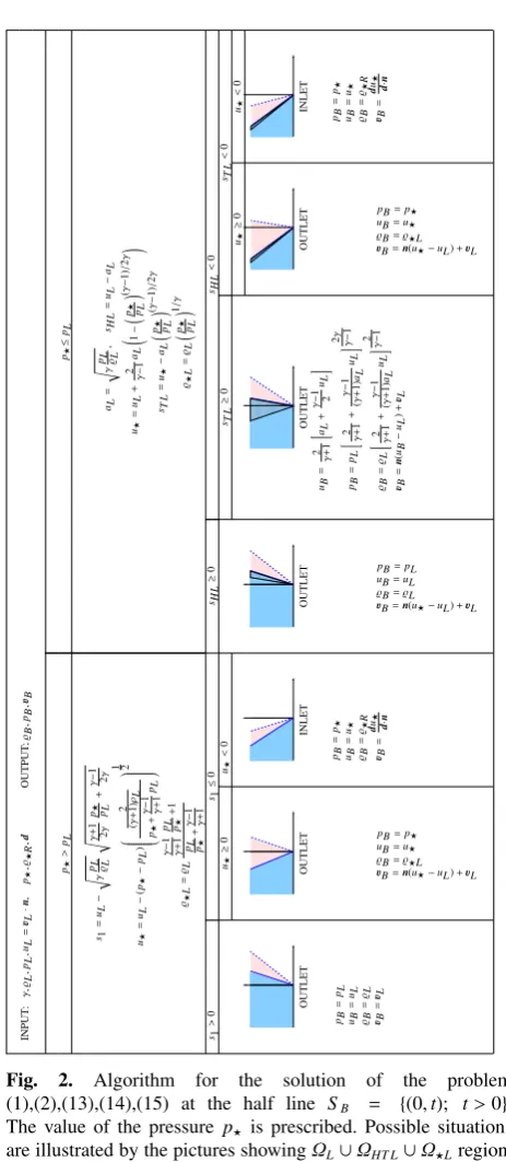
solu-tion of the Riemann problem for the split Euler equasolu-tions, shown in Section 2. This way we have prescribed the de-sired pressure value whenever it is possible (see the general form of the solution in Section 2). Now it is possible to use (4),(5),(6) Further we must discuss all the possibilities of the left (shock, rarefaction) and the middle (discontinuity) wave in the solution, which is shown in ﬁgure 2. In the case ofoutlet(u ≥0), the transformation of the velocity into the global coordinates is

uB=n(uB−uL)+uL.

HereuB denotes the computed velocity in the normal

di-rection. In the case of aninlet(u<0) we mustprescribe

another conditionsin order to obtain a uniquely solvable system. Here we may choose (for example) arbitrary den-sityGIVENand the direction of the velocityd.

R =GIVEN, uB=d|u|, with uB·n=u (15)

Then it is

pB =pGIVEN, B=GIVEN, uB= d

u

d·n.

The analysis of this problem was shown also in [8].

INPUT : γ, L , pL , uL = uL · n , p , R , d OUTPUT ; B , pB , uB p > pL p ≤ pL s1 = uL − γ pLL γ

+

1

2

γ

ppL

+ γ − 1 2 γ u = uL − ( p − pL ) ⎛ ⎜ ⎜ ⎜ ⎜ ⎜ ⎜ ⎜ ⎜ ⎜ ⎝ 2 ( γ + 1) ρL p + γ − 1 γ + 1 pL ⎞ ⎟ ⎟ ⎟ ⎟ ⎟ ⎟ ⎟ ⎟ ⎟ ⎠ 1 2 L = L γ − 1 γ + 1

pLp

+

1

pL p

+ γ − 1 γ + 1 aL = γ pL,L

s HL = uL − aL u = uL + 2 γ − 1 aL 1−

pp

L (γ− 1) / 2 γ s TL = u − aL ppL (γ− 1) / 2 γ L = L pp

L 1/γ s1 > 0 s1 ≤ 0 s HL ≥ 0 s HL < 0 u ≥ 0 u < 0 s TL ≥ 0 s TL < 0 u ≥ 0 u < 0 OUTLET OUTLET INLET 000000000000000000000000000000000000000000000000000000000000000000000000000000000000000000000000000000000000000000000000000000000000000000000000000000000000000000000000000000000000000000000000000000000000000000000000000000000000000000000000000000000000000000000000000000000000000000000000000000 111111111111111111111111111111111111111111111111111111111111111111111111111111111111111111111111111111111111111111111111111111111111111111111111111111111111111111111111111111111111111111111111111111111111111111111111111111111111111111111111111111111111111111111111111111111111111111111111111111 OUTLET 00000000000000000000000000000000000000000000000000000000000000000000000000000000000000000000000000000000000000000000000000000000000000000000000000000000000000000000000000000000000000000000000000000000000000000000000000000000000000000000000000000000000000000000000000000000000000000000000000000000000000000000000000000000000000000000000000000000000000000000000000000000000000000000000000000000000000000000000000000000000000000000000000000000000000000000000000000000000000000 11111111111111111111111111111111111111111111111111111111111111111111111111111111111111111111111111111111111111111111111111111111111111111111111111111111111111111111111111111111111111111111111111111111111111111111111111111111111111111111111111111111111111111111111111111111111111111111111111111111111111111111111111111111111111111111111111111111111111111111111111111111111111111111111111111111111111111111111111111111111111111111111111111111111111111111111111111111111111111 OUTLET 000000000000000000000000000000000000000000000000000000000000000000000000000000000000000000000000000000000000000000000000000000000000000000000000000000000000000000000000000000000000000000000000000000000000000000000000000000000000000000000000000000000000000000000000000000000000000000000000000000000000000000000000000000000000000000000000000000000000000000000000000000000000000000000000000000000000000000000000000000000000000000000000000000000000000000000000000000000000000000000000000000000000000000000000000000000000000000000000000000000000000000000000000000000000000000000000000000000000000000000000000000000000000000000000000000000000000000000000000000000000000000000000000000000000000000000000000000000000000000000000000000000000000000000000000000000000000000000000000000 111111111111111111111111111111111111111111111111111111111111111111111111111111111111111111111111111111111111111111111111111111111111111111111111111111111111111111111111111111111111111111111111111111111111111111111111111111111111111111111111111111111111111111111111111111111111111111111111111111111111111111111111111111111111111111111111111111111111111111111111111111111111111111111111111111111111111111111111111111111111111111111111111111111111111111111111111111111111111111111111111111111111111111111111111111111111111111111111111111111111111111111111111111111111111111111111111111111111111111111111111111111111111111111111111111111111111111111111111111111111111111111111111111111111111111111111111111111111111111111111111111111111111111111111111111111111111111111111111111 OUTLET 000000000000000000000000000000000000000000000000000000000000000000000000000000000000000000000000000000000000000000000000000000000000000000000000000000000000000000000000000000000000000000000000000000000000000000000000000000000000000000000000000000000000000000000000000000000000000000000000000000000000000000000000000000000000000000000000000000000000000000000000000000000000000000000000000000000000000000000000000000000000000000000000000000000000000000000000000000000000000000000000000000000000000000000000000000000000000000000000000000000000000000000000000000000000000000000000000000000000000000000000000000000000000000000000000000000000000000000000000000000000000000000000000000000000000000000000000000000000000000000000000000000000000000000000000000000000000000000000000000 111111111111111111111111111111111111111111111111111111111111111111111111111111111111111111111111111111111111111111111111111111111111111111111111111111111111111111111111111111111111111111111111111111111111111111111111111111111111111111111111111111111111111111111111111111111111111111111111111111111111111111111111111111111111111111111111111111111111111111111111111111111111111111111111111111111111111111111111111111111111111111111111111111111111111111111111111111111111111111111111111111111111111111111111111111111111111111111111111111111111111111111111111111111111111111111111111111111111111111111111111111111111111111111111111111111111111111111111111111111111111111111111111111111111111111111111111111111111111111111111111111111111111111111111111111111111111111111111111111 INLET pB = pL uB = uL B = L uB = uL pB=p uB=u

B=L uB=n(u−uL)+uL pB = p uB = u B = R uB = d

u _d·n pB=pL uB=uL

B=L uB=n(u−uL)+uL uB

=

2 _γ+1

aL

+

γ

−

1u₂

L

pB

=

pL 2 γ+

1 + γ − 1 ( γ + 1) aL uL 2 γ γ − 1 B = L 2 γ+

1 + γ − 1 ( γ + 1) aL uL

2 _γ−1

uB = n ( uB − uL ) + uL pB=p uB=u

B=L uB=n(u−uL)+uL pB = p uB = u B = R uB = d

u _d·n

Fig. 2. Algorithm for the solution of the problem (1),(2),(13),(14),(15) at the half line SB = {(0,t); t>0}.

The value of the pressure p is prescribed. Possible situations are illustrated by the pictures showingΩL∪ΩHT L∪ΩLregion.

The sought boundary state located at the time axis, marked red.

input data solution

Test uL p B uB pB

1 1.0 4.57991 1 -0.50000 4.57991

2 -1.0 0.12913 0.23175 0.50000 0.12913

3 2.0 0.5 1.0 2.0 1.0

4 2.0 3.0 1.0 2.0 1.0

5 2.0 6.77045 3.2593 0.00002 6.77045

6 2.0 8.0 1 -0.23607 8.0

(5)

4 Boundary Condition by Preference of

Velocity

Here we show the boundary condition prefering the pre-scribed given velocity at the face. The conservation laws must be satisﬁed in close vicnity to the boundary face. Therefore we use the analysis of the incomplete Riemann problem to construct the values for the density and the velocity at each boundary face. The following notation is used (some values are used only for an INLET case)

at time 0,uL=uL·n

uGIVEN given velocity vector (=desired value at the face)

uGIVENgiven value for the normal vcomponent of

veloc-ity (=desired normal velocity at the face)

uGIVEN=uGIVEN·n

and thecomplementary conditions(prescribed normal

com-ponent of velocity).

u=uGIVEN, (16)

uR=u, (17)

Hereudenotes the normal component of velocity inΩL∪

ΩR part of the solution of the Riemann problem for the

split Euler equations, shown in Section 2. This way we have prescribed the desired normal component of velocity whenever it is possible (see the general form of the solution in Section 2). Now it is possible to use (12),(5),(6). Further we must discuss all the possibilities of the left (shock, rar-efaction) and the middle (discontinuity) wave in the solu-tion, which is shown in ﬁgure 3. The tangential velocities

are conserved (same as “left” values) in the case ofoutlet

(u ≥0), and the velocity vector in the global coordinates

is

uB=n(uB−uL)+uL.

HereuB denotes the computed velocity in the normal

di-rection. In the case of aninlet(u<0) we mustprescribe

another conditionsin order to obtain a uniquely solvable system. Here we may choose (for example) arbitrary den-sityGIVENand the whole vector of velocity

R=GIVEN, uR =uGIVEN. (18)

For example, it is possible to choose the densityR

us-ing the given entropy index po

oγ (po, oare some reference

values for the pressure and the density)

R =p1/γ/

po

γo

1/γ

=o

p

po

1/γ

Another possibility is to conserve (choose) the total

temperature θ0 for the inlet case. Then, using

thermody-namic relations (energy equation for a perfect gas), it is

R =

p

Rθ0 1−γ−₂1|uGIVEN|

2

γRθ0

. (19)

Letθ0 = θ0R = pR/(RR 1+γ−₂1 |uR|

2

γpR/R

) anduGIVEN =uR.

Then, using (19), it isR=Rp_p_R.

The algorithm for the construction of the primitive

vari-ablesB,uB,pBat the boundary face is shown in Fig. 3. The

complete analysis of this problem is shown in [8].

INPUT : γ, L , pL , uL = uL · n , u = uR · n , R , uR OUTPUT ; B , pB , uB u < uL u ≥ uL D = 4 L γ pL +

2(L

γ

+

1)2₂

( uL − u )2 p = 1 2 2p L + γ − 1 2 L ( uL − u )2 + ( uL − u ) √ D s1 = uL − γ pL L γ

+

1

2

γ

p pL

+ γ − 1 2 γ L = L γ − 1 γ + 1

pL p

+

1

pLp

+ γ − 1 γ + 1 aL = γ pL,L

s HL = uL − aL p = pL ⎛ ⎜ ⎜ ⎜ ⎜ ⎜ ⎜ ⎜ ⎜ ⎝− u + uL + 2 γ − 1 aL 2 γ − 1 aL ⎞ ⎟ ⎟ ⎟ ⎟ ⎟ ⎟ ⎟ ⎟ ⎠ 2 γ γ − 1 s TL = u − aL pp

L (γ− 1) / 2 γ L = L pp

L 1/γ s1 ≥ 0 s1 < 0 s HL ≥ 0 s HL < 0 u ≥ 0 u < 0 s TL ≥ 0 s TL < 0 u ≥ 0 u < 0 OUTLET OUTLET INLET 000000000000000000000000000000000000000000000000000000000000000000000000000000000000000000000000000000000000000000000000000000000000000000000000000000000000000000000000000000000000000000000000000000000000000000000000000000000000000000000000000000000000000000000000000000000000000000000000000000 111111111111111111111111111111111111111111111111111111111111111111111111111111111111111111111111111111111111111111111111111111111111111111111111111111111111111111111111111111111111111111111111111111111111111111111111111111111111111111111111111111111111111111111111111111111111111111111111111111 OUTLET 00000000000000000000000000000000000000000000000000000000000000000000000000000000000000000000000000000000000000000000000000000000000000000000000000000000000000000000000000000000000000000000000000000000000000000000000000000000000000000000000000000000000000000000000000000000000000000000000000000000000000000000000000000000000000000000000000000000000000000000000000000000000000000000000000000000000000000000000000000000000000000000000000000000000000000000000000000000000000000 11111111111111111111111111111111111111111111111111111111111111111111111111111111111111111111111111111111111111111111111111111111111111111111111111111111111111111111111111111111111111111111111111111111111111111111111111111111111111111111111111111111111111111111111111111111111111111111111111111111111111111111111111111111111111111111111111111111111111111111111111111111111111111111111111111111111111111111111111111111111111111111111111111111111111111111111111111111111111111 OUTLET 000000000000000000000000000000000000000000000000000000000000000000000000000000000000000000000000000000000000000000000000000000000000000000000000000000000000000000000000000000000000000000000000000000000000000000000000000000000000000000000000000000000000000000000000000000000000000000000000000000000000000000000000000000000000000000000000000000000000000000000000000000000000000000000000000000000000000000000000000000000000000000000000000000000000000000000000000000000000000000000000000000000000000000000000000000000000000000000000000000000000000000000000000000000000000000000000000000000000000000000000000000000000000000000000000000000000000000000000000000000000000000000000000000000000000000000000000000000000000000000000000000000000000000000000000000000000000000000000000000 111111111111111111111111111111111111111111111111111111111111111111111111111111111111111111111111111111111111111111111111111111111111111111111111111111111111111111111111111111111111111111111111111111111111111111111111111111111111111111111111111111111111111111111111111111111111111111111111111111111111111111111111111111111111111111111111111111111111111111111111111111111111111111111111111111111111111111111111111111111111111111111111111111111111111111111111111111111111111111111111111111111111111111111111111111111111111111111111111111111111111111111111111111111111111111111111111111111111111111111111111111111111111111111111111111111111111111111111111111111111111111111111111111111111111111111111111111111111111111111111111111111111111111111111111111111111111111111111111111 OUTLET 000000000000000000000000000000000000000000000000000000000000000000000000000000000000000000000000000000000000000000000000000000000000000000000000000000000000000000000000000000000000000000000000000000000000000000000000000000000000000000000000000000000000000000000000000000000000000000000000000000000000000000000000000000000000000000000000000000000000000000000000000000000000000000000000000000000000000000000000000000000000000000000000000000000000000000000000000000000000000000000000000000000000000000000000000000000000000000000000000000000000000000000000000000000000000000000000000000000000000000000000000000000000000000000000000000000000000000000000000000000000000000000000000000000000000000000000000000000000000000000000000000000000000000000000000000000000000000000000000000 111111111111111111111111111111111111111111111111111111111111111111111111111111111111111111111111111111111111111111111111111111111111111111111111111111111111111111111111111111111111111111111111111111111111111111111111111111111111111111111111111111111111111111111111111111111111111111111111111111111111111111111111111111111111111111111111111111111111111111111111111111111111111111111111111111111111111111111111111111111111111111111111111111111111111111111111111111111111111111111111111111111111111111111111111111111111111111111111111111111111111111111111111111111111111111111111111111111111111111111111111111111111111111111111111111111111111111111111111111111111111111111111111111111111111111111111111111111111111111111111111111111111111111111111111111111111111111111111111111 INLET pB = pL uB = uL uB = uL B = L

pB=p uB=u

B=L uB=n(u−uL)+uL pB = p uB = u uB = uR B = R pB = pL uB = uL uB = uL B = L pB = pL 2 γ+

1 + γ − 1 ( γ + 1) aL uL 2 γ γ − 1 uB =

2 _γ+1

aL

+

γ

−

1u₂

L uB = n ( uB − uL ) + uL B = L 2 γ+

1 + γ − 1 ( γ + 1) aL uL

2 _γ−1

pB=p uB=u

B=L uB=n(u−uL)+uL pB = p uB = u uB = uR B = R

Possible situations are illustrated by the pictures showing the regionΩL∪ΩHT L∪ΩLwith the sought boundary state located

(6)

5 Boundary Condition by Preference of

Temperature

Using this boundary condition, we try to prescribe given static temperature at the face, comlete analysis was shown in [8]. The conservation laws must be satisﬁed in close vicnity to the boundary face. We use the analysis of the incomplete Riemann problem to construct the values for the density, pressure and velocity. The following notation is used (some values are used only for an INLET case)

at time 0,uL=uL·n

θGIVEN given value for the pressure (=desired

tempera-ture at the face)

and thecomplementary conditions(prescribed pressure).

θL=θGIVEN, (20)

θR=θL, (21)

HereθLdenotes the static temperature inΩLpart of the

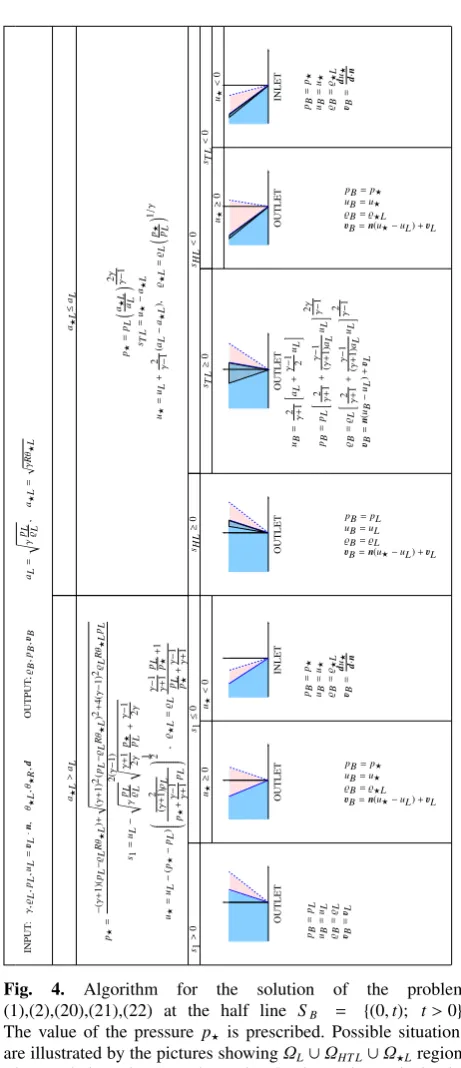
solution of the Riemann problem for the split Euler equa-tions, shown in Section 2. This way we have prescribed the desired temperature value whenever it is possible (see the general form of the solution in Section 2). Now it is pos-sible to use (4),(5),(6) together with the equation of state

L= RpθL.We must discuss all the possibilities of the left

(shock, rarefaction) and the middle (discontinuity) wave in

the solution, which is shown in ﬁgure 4. In the case of

out-let(u ≥ 0), the transformation of the velocity into the

global coordinates is

uB=n(uB−uL)+uL.

HereuBdenotes the computed velocity in the normal

direc-tion. In the case of aninlet(u<0) we use the condition

(21), which ensures that pR = p,uR = u, R = R =

L.Further it is possible to prescribe the direction of the

velocityd

uB=d|u|, with uB·n=u. (22)

Then it is

uB= d

u

d·n.

INPUT : γ, L , pL , uL = uL · n ,θ L ,θ R , d OUTPUT ; B , pB , uB aL = γ pL,L

a

L

=

γ

R

θ L

a L > aL a L ≤ aL p = − ( γ + 1)( pL − L R

θ L

)

+

(γ

+

1)

2(p

L

−

L

R

θ L

)2 + 4( γ − 1) 2 L R

θ L

pL 2( γ − 1) s1 = uL − γ pLL γ

+

1

2

γ

ppL

+ γ − 1 2 γ u = uL − ( p − pL ) ⎛ ⎜ ⎜ ⎜ ⎜ ⎜ ⎜ ⎜ ⎜ ⎜ ⎝ 2 ( γ + 1) ρL p + γ − 1 γ + 1 pL ⎞ ⎟ ⎟ ⎟ ⎟ ⎟ ⎟ ⎟ ⎟ ⎟ ⎠

1 2 ,

L = L γ − 1 γ + 1

pLp

+

1

pLp

+ γ − 1 γ + 1 p = pL a L aL 2 γ γ − 1 s TL = u − a L u = uL + 2 γ − 1 ( aL − a L ) , L = L pp

L 1/γ s1 > 0 s1 ≤ 0 s HL ≥ 0 s HL < 0 u ≥ 0 u < 0 s TL ≥ 0 s TL < 0 u ≥ 0 u < 0 OUTLET OUTLET INLET 000000000000000000000000000000000000000000000000000000000000000000000000000000000000000000000000000000000000000000000000000000000000000000000000000000000000000000000000000000000000000000000000000000000000000000000000000000000000000000000000000000000000000000000000000000000000000000000000000000 111111111111111111111111111111111111111111111111111111111111111111111111111111111111111111111111111111111111111111111111111111111111111111111111111111111111111111111111111111111111111111111111111111111111111111111111111111111111111111111111111111111111111111111111111111111111111111111111111111 OUTLET 00000000000000000000000000000000000000000000000000000000000000000000000000000000000000000000000000000000000000000000000000000000000000000000000000000000000000000000000000000000000000000000000000000000000000000000000000000000000000000000000000000000000000000000000000000000000000000000000000000000000000000000000000000000000000000000000000000000000000000000000000000000000000000000000000000000000000000000000000000000000000000000000000000000000000000000000000000000000000000 11111111111111111111111111111111111111111111111111111111111111111111111111111111111111111111111111111111111111111111111111111111111111111111111111111111111111111111111111111111111111111111111111111111111111111111111111111111111111111111111111111111111111111111111111111111111111111111111111111111111111111111111111111111111111111111111111111111111111111111111111111111111111111111111111111111111111111111111111111111111111111111111111111111111111111111111111111111111111111 OUTLET 000000000000000000000000000000000000000000000000000000000000000000000000000000000000000000000000000000000000000000000000000000000000000000000000000000000000000000000000000000000000000000000000000000000000000000000000000000000000000000000000000000000000000000000000000000000000000000000000000000000000000000000000000000000000000000000000000000000000000000000000000000000000000000000000000000000000000000000000000000000000000000000000000000000000000000000000000000000000000000000000000000000000000000000000000000000000000000000000000000000000000000000000000000000000000000000000000000000000000000000000000000000000000000000000000000000000000000000000000000000000000000000000000000000000000000000000000000000000000000000000000000000000000000000000000000000000000000000000000000 111111111111111111111111111111111111111111111111111111111111111111111111111111111111111111111111111111111111111111111111111111111111111111111111111111111111111111111111111111111111111111111111111111111111111111111111111111111111111111111111111111111111111111111111111111111111111111111111111111111111111111111111111111111111111111111111111111111111111111111111111111111111111111111111111111111111111111111111111111111111111111111111111111111111111111111111111111111111111111111111111111111111111111111111111111111111111111111111111111111111111111111111111111111111111111111111111111111111111111111111111111111111111111111111111111111111111111111111111111111111111111111111111111111111111111111111111111111111111111111111111111111111111111111111111111111111111111111111111111 OUTLET 000000000000000000000000000000000000000000000000000000000000000000000000000000000000000000000000000000000000000000000000000000000000000000000000000000000000000000000000000000000000000000000000000000000000000000000000000000000000000000000000000000000000000000000000000000000000000000000000000000000000000000000000000000000000000000000000000000000000000000000000000000000000000000000000000000000000000000000000000000000000000000000000000000000000000000000000000000000000000000000000000000000000000000000000000000000000000000000000000000000000000000000000000000000000000000000000000000000000000000000000000000000000000000000000000000000000000000000000000000000000000000000000000000000000000000000000000000000000000000000000000000000000000000000000000000000000000000000000000000 111111111111111111111111111111111111111111111111111111111111111111111111111111111111111111111111111111111111111111111111111111111111111111111111111111111111111111111111111111111111111111111111111111111111111111111111111111111111111111111111111111111111111111111111111111111111111111111111111111111111111111111111111111111111111111111111111111111111111111111111111111111111111111111111111111111111111111111111111111111111111111111111111111111111111111111111111111111111111111111111111111111111111111111111111111111111111111111111111111111111111111111111111111111111111111111111111111111111111111111111111111111111111111111111111111111111111111111111111111111111111111111111111111111111111111111111111111111111111111111111111111111111111111111111111111111111111111111111111111 INLET pB = pL uB = uL B = L uB = uL pB=p uB=u

B=L uB=n(u−uL)+uL pB = p uB = u B = L uB = d

u _d·n pB=pL uB=uL

B=L uB=n(u−uL)+uL uB = 2 γ + 1 aL + γ − 1 2 uL pB = pL 2 γ+

1 + γ − 1 ( γ + 1) aL uL 2 γ γ − 1 B = L

2 γ+

1 + γ − 1 ( γ + 1) aL uL 2 γ − 1 uB = n ( uB − uL ) + uL pB=p uB=u

B=L uB=n(u−uL)+uL pB = p uB = u B = L uB = d

u _d·n

The value of the pressure p is prescribed. Possible situations are illustrated by the pictures showingΩL∪ΩHT L∪ΩLregion.

The sought boundary state located at the time axis, marked red.

input data solution (rounded)

uL θL B uB pB θB

0.0 4500.0 7.0492 -2434.5 9105332.5 4500.0 0.0 300.00 1.5000 -62.370 129171.2 300.00 0.0 270.00 1.1547 26.345 89486.3 270.00 0.0 200.00 0.54528 255.83 31303.2 200.00 0.0 100.00 0.50235 278.89 27908.2 193.55 200.0 240.00 0.88342 312.22 61512.3 242.58 200.0 260.00 1.0507 257.13 78413.4 260.00

Table 2.The initial datauL, θLand the solutionB,uB,pB for

(7)

6 Boundary Condition by Preference of

Total Quantities and Direction of Velocity

Using this boundary condition, we try to prescribe given total quantities at the face, comlete analysis was shown in [8], [5]. The conservation laws must be satisﬁed in close vicnity to the boundary face. We use the analysis of the incomplete Riemann problem to construct the values for the density, pressure and velocity. The following notation is used (some values are used only for an INLET case)

at time 0,uL=uL·n

po given value for the total pressure (=desired total

pressure at the face)

θo given value for the total temperature (=desired

to-tal temperature at the face)

and thecomplementary conditions(prescribed direction

of velocity and given total quantities).

uB=d|uB|, with uB·n=u. (23)

θR=θo

1−γ−1

2a2

o

u2

, with a2₀=γRθ0(d·n)2, (24)

p=po

θR

θ0

γ/(γ−1)

(25)

u<0. (26)

Hereθo > 0,po > 0 are given constants, R denotes the

characteristic gas constant, andγis the adiabatic constant.

The equations (24),(25) are considered for the velocityu∈

− 2a2

o (γ−1),

2a2

o (γ−1)

. The equations (24),(25) come from the

idea, that thetotal pressure poand thetotal temperatureθo

are known (prescribed) in the regionΩR.

According to analysis shown in [5], there are two

pos-sibillities for the 1-wave, either there is a1-shock wave

and the sought velocityucan be found as a root of the

function

F(u)=po

1−γ−1 2a2

o

u2

γ/(γ−1)

−PS(u), (27)

considered foru<uL,−

2a2

o

(γ−1) <u <0,and withPS(u)

deﬁned in (12).

Or there is a1-rarefaction wave, and the velocityu

can be computed combining (24),(25),(12) as

u= 2 uL+

2 γ−1aL

−√DIS

2

1+ 2a2L

(γ−1)a2

o

po

pL

(γ−1)/γ, (28)

DIS=4

po pL

_(γ₋_1)/γ ₂a2

L

(γ−1)a2o ⎡ ⎢⎢⎢⎢⎢ ⎢⎢⎣ 2a2o

(γ−1)+ 4a2

L

(γ−1)2

po pL

_(γ₋_1)/γ −

uL+_γ2aL₋₁

2⎤_{⎥⎥⎥⎥⎥}

⎥⎥⎦.

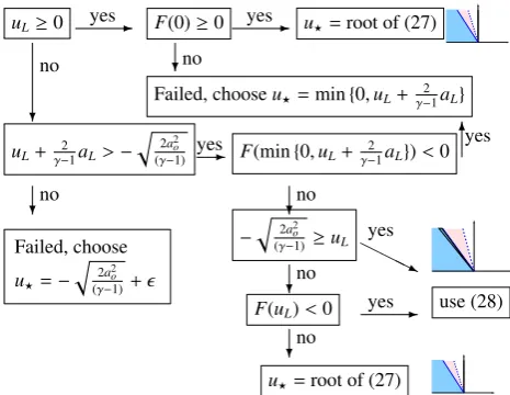
Summarizing the above possibilities of the 1-shock and the 1-rarefaction wave we can construct the algorithm in

ﬁgure 5. for the computation of the velocityuin thestar

region.

-yes

uL≥0

?

no

F(0)≥0 yes- u=root of (27)

?no

Failed, chooseu=min{0,uL+_γ₋21aL}

uL+_γ₋21aL>−

2a2

o

(γ−1) yes- F(min{0,uL+

2

γ−1aL})<0

6yes

?no

Failed, choose

u=−

2a2

o

(γ−1)+

− 2a2

o

(γ−1) ≥uL

HHHjyes 000000000000000000000000000000000000000000000000000000000000000000000000000000000000000000000000000000000000000000000000000000000000000000000000000000000000000000000000000000000000000000000000000000000000000000000000000000000000000000000000000000000000000000000000000000000000000000000000000000000000000000000000000000000000000000000000000000000000000000000000000000000000000000000000000000000000000000000000000000000000000000000000000000000000000000000000000000000000000000000000000000000000000000000000000000000000000000000000000000000000000000000000000000000000000000000000000000000000000000000000000000000000000000000000000000000000000000000000000000000000000000000000000000000000000000000000000000000000000000000000000000000000000000000000000000000000000000000000000000 111111111111111111 111111111111111111 111111111111111111 111111111111111111 111111111111111111 111111111111111111 111111111111111111 111111111111111111 111111111111111111 111111111111111111 111111111111111111 111111111111111111 111111111111111111 111111111111111111 111111111111111111 111111111111111111 111111111111111111 111111111111111111 111111111111111111 111111111111111111 111111111111111111 111111111111111111 111111111111111111 111111111111111111 111111111111111111 111111111111111111 111111111111111111 111111111111111111 111111111111111111 111111111111111111 111111111111111111 111111111111111111 111111111111111111 111111111111111111 111111111111111111 111111111111111111 111111111111111111 111111111111111111 111111111111111111 111111111111111111 111111111111111111 111111111111111111 111111111111111111

?no

F(uL)<0 yes- use (28)

?no

u=root of (27)

Fig. 5.Algorithm for the velocity solutionu <0.In the case of failure, the problem doesn’t have a solution, and the values are chosen.

Knowing the velocityuwe compute the pressure p

using (25), and the densityR = _Rp_θ_R.At last we set the

boundary values as

pB=p, B=R, uB= d

u

d·n.

The problem (1),(2), (25), (24) has a unique solution for

the initial data satisfyinguL+_γ2₋₁aL>−

2a2

o

(γ−1), andF(min{0,uL+

2

γ−1aL})>0.In the case ofuL+

2

γ−1aL≤ −

2a2

o

(γ−1) there is

no solution. In this case we prescribe the velocity u =

− 2a2

o

(γ−1) +,with > 0 being a small positive constant.

If F(min{0,uL+ _γ2₋₁aL}) ≤ 0 then the problem does not

have a negative solution, and for the practical applications

we choose the velocity u = min{0,uL+ _γ2₋₁aL}, or we

use the boundary condition preferring the static pressure

p=po, see [2, 8], in this case.

Let ˜p0,θ˜0 be the given total quantities together with the

giventangential velocity components:vtandwtare the

velocity components in the direction ofoandp. Hereo·n=

0,|o|=1,andp=n×o.Then we set

d=−n, θ0=θ˜o−γ−

1

2γR (v

2

t +w2t), p0=p˜0

θ0

˜

θ0

γ

γ−1

,

and we use the same algorithm (ﬁgure 5.) for the

compu-tation of the velocityu.Then it is pB = p, B =R,

and

(8)

7 Inlet Boundary Condition by Preference

of Massﬂow

Using this boundary condition, we try to prescribe given total quantities at the face, comlete analysis was shown in [7]. The conservation laws must be satisﬁed in close vic-nity to the boundary face. We use the analysis of the in-complete Riemann problem to construct the values for the density, pressure and velocity. The following notation is used (some values are used only for an INLET case)

B static density at the boundary (unknown) pB static pressure at the boundary (unknown)

uB velocity vector at the boundary (in global coordi-nates) (unknown)

uB normal component of velocity at the boundary (lo-cal coordinates) (unknown)

L static density near the wall, time 0 pL static pressure near the wall, time 0

uL velocity vector, state near the wall at time 0 uL normal component of velocity, state near the wall

at time 0,uL=uL·n

G given inlet massﬂow (=desired massﬂow at the face)

θ0 given value for the total temperature (=desired

to-tal temperature at the face)

At the vicinity of the boundary we solve the modiﬁed Rie-mann problem for the split Euler equations (1), introduced in Section 2, with the left-hand side initial condition (2) and thecomplementary conditionsprescribing the mass ﬂow,direction of velocity, and total temperature inΩR given as

uR =G, (29)

uB=d|uB|, with uB·n=u. (30)

θR=θo

1−γ−1 2a2

o u2

, with a2₀=γRθ0(d·n)2, (31)

u<0, (32)

whereG ≤ 0 is given constant (G = mass f lo_{f ace area}w). Hereγ andRare gas constants. The equation (31) is considered for

the velocityu ∈

− 2a2 o

(γ−1),0

. In general, there are two possibilities of the wave pattern, which may interest us. We seek the unknown velocityuas a root of the function

F(u)=G(u)−G, whereG(u)=u P(u)

Rθ(u), (33) withP(u) deﬁned in (12), and

θ(u)=θ0

⎛

⎜⎜⎜⎜⎝1−γ−1 2

u2

a2 0

⎞ ⎟⎟⎟⎟⎠, u∈

⎛ ⎜⎜⎜⎜⎜ ⎜⎜⎝−

2a2

0

γ−1,0 ⎞ ⎟⎟⎟⎟⎟ ⎟⎟⎠.

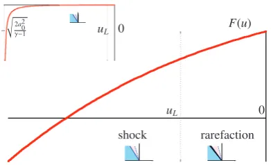
The ﬁgure 6. shows example of such function for the cho-sen values. The function F(u) is monotone, and it has a

unique root ifuL+_γ2₋₁aL>−

2a2 0 γ−1.

Once the velocityu < 0 is known, it is possible to compute the remaining values

B=G/u, pB=p(u),uB= d u

d·n.

0 uL

shock rarefaction F(u)

−

2a2 0

γ−1 uL 0

Fig. 6.Graph of the functionF(u) (red line) for given valuesθ0=

273.15, γ=1.4, L=1.25,pL=100000,uL=−50,G=−200.

uL+_γ₋21aL>−

2a2 0

γ−1 yes- u=root of (33)

?no

ERROR, NO SOLUTION. Low temperatureθ0at the inlet.

Fig. 7.Algorithm for the velocity solutionu <0.In the case of

failure, the problem doesn’t have a solution, and the values are chosen.

Let ˜θ0be the given total temperature together with the given tangential velocity components:vtandwtare the veloc-ity components in the direction ofoandp. Hereo·n=0, |o|=1,andp=n×o.Then we set

d=−n, θ0=θ˜o−γ−

1

2γR(v2t +w2t),

and we use the same algorithm (ﬁgure 7.) for the compu-tation of the velocityu.Then it is pB = p, B =R, and

B=G/u, pB =p(u),

uB=(n1u+o1vt+p1wt,n2u+o2vt+p2wt,n3u+o3vt+p3wt,).

input data solution

uL pL G B u p

40 70000 -44.3198 1.2853 -34.481 100558.8 -100 70000 -171.582 1.1693 -146.74 88080.1 -200 100000 -185.547 1.1427 -162.38 85285.7 -300 70000 -244.851 0.89857 -272.49 60920.9 -600 70000 -207.065 0.49508 -418.24 26444.9

Table 3.The initial datauL,pL,Gand the solutionB,u, p

(9)

8 Outlet Boundary Condition by

Preference of Massﬂow

Using this boundary condition, we try to prescribe given total quantities at the face, comlete analysis was shown in [6, 7]. The conservation laws must be satisﬁed in close vic-nity to the boundary face. We use the analysis of the in-complete Riemann problem to construct the values for the density, pressure and velocity. The following notation is used (some values are used only for an INLET case)

B static density at the boundary (unknown) pB static pressure at the boundary (unknown)

uB velocity vector at the boundary (in global coordi-nates) (unknown)

uB normal component of velocity at the boundary (lo-cal coordinates) (unknown)

L static density near the wall, time 0 pL static pressure near the wall, time 0

uL velocity vector, state near the wall at time 0 uL normal component of velocity, state near the wall

at time 0,uL=uL·n

G given inlet massﬂow (=desired massﬂow at the face)

At the vicinity of the boundary we solve the modiﬁed Rie-mann problem for the split Euler equations (1), introduced in Section 2, with the left-hand side initial condition (2) and thecomplementary conditionsprescribing the mass ﬂow

uR =G, (34)

whereG ≥0 is given constant (G = mass f lo_{f ace area}w). We are interested in the solution withu>0, andsL?<0,which

guarantees the possibility of the values to be prescribed at the boundary. In general, there are two possibilities of the wave pattern, which may interest us.

– 1-shock wave

Here, we are interested in the solution withs1<0,u>

0.Let us construct the functionFS(u), using the rela-tions (4),(5)

FS(u)=uL(u)−G, (35)

where

L(u)=L

(γ−1)pL+(γ+1)PS(u) (γ+1)pL+(γ−1)PS(u),

and PS(u) deﬁned in (12). The sought velocityu is

the root of this function FS(u). It iss1 < 0 foru <

uX =uL2+(γ−1)M

2 L

(γ+1)M2

L ,

withM2

L=u2L/γp,see [8]. The ﬁrst derivative isF_S >0 foru <min{uL,uX}. The problem has a solution with the 1-shock wave ifFS(min{uL,uX})> 0.

– 1-rarefaction wave

Let us assume the solution with the 1-rarefaction wave. Using (4),(5),(34), the velocity u is the root of the function

FR(u)=uL

1−γ−1 2aL

(u−uL)

2

γ−1

−G, (36)

deﬁned in the intervaluL<u<uL+_γ2₋aL₁.It isFR(uL)= LuL−G. The ﬁrst derivative is zero at the pointsu1=

uL+_γ2₋aL₁, u0= _γγ₊−1₁ uL+_γ2a₋L₁

. DerivativeF_R(u)>0 in the interval (0,u0) andF(u)<0 foru ∈(u0,u1).The

maximum of the functionFRis at the pointu0. We are

interested in the solution withsT L<0. This is satisﬁed only foy u<u0.

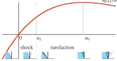
0 uL u0

shock rarefaction

uL(u)

Fig. 8.Example of the function uL(u), hereuL = 20, γ =

1.4, L=1.25,pL=100000.

Algorithm

Here we present the possible algorithm for the solution of the sought values at the boundary.

F(uL)=uLL−G i f F(uL)>0 t h e n

u= r o o t o f FS(u), u∈(0,min{uX,uL}), (35) .

e l s e

i f uL>u0 t h e n

u=uL

e l s e i f (u1<u0)

u=u1−ε

e l s e

i f F(u0)<0 t h e n

u=u0

e l s e

u= r o o t o f FR(u), u∈(uL,u0), (36) .

end e n d i f end end

Compute pB=p, B=L u s i n g (12),(5).

The resulting boundary velocity in the global coordi-nates isuB=n(uB−uL)+uL.

input data solution

uL G GB B uB pB

-20 1 1.00 1.174034 0.8517646 91596.49 -20 50 50.00 1.011280 49.44231 74326.85 -20 150 130.35 0.4730351 275.5533 25655.28 20 1 1.00 1.323527 0.7555568 108333.1 20 100 100.00 0.9684777 103.2548 69960.27 20 200 150.45 0.5330942 282.2200 30328.54 400 10.0 10.00 3.218839 3.106711 421919.0 400 100 100.00 3.059145 32.68887 385170.7

400 600 500 1.25 400 100000

Table 4.Outlet boundary condition by preference of massﬂow.

(10)

9 EXAMPLES

9.1 The Flow Around the Obstacle

Here we present a computational result of the 2D

non-stationary inviscid channel ﬂow at Mach numberM=0.67.

A body immersed in the flowing fluid establishes a certain wave pattern which evolves in time and eventually exits the channel. At figure 1 we show, that the fixed (values are fixed at the boundary) and linearized (as described in [9]) boundary conditions do not give the expected result in time. The inlet is located left, outlet right, other boundaries are considered as wall. The fixed boundary conditions give incorrect results near boundaries. The linearized boundary condition reflects the waves into the domain, leading to the oscillations in the solution. The new suggested boundary

conditions do not suﬀer from these drawbacks. The

resid-ual behavior (shown right) demonstrates this result.

Fig. 9.Incompressible ﬂow, body in the channel. Comparison of the various boundary conditions.

9.2 The Shortened Domain Example

The following numerical example shows superior behav-ior of the suggested boundary condition. This is the test case of the the inviscid ﬂow through the Double Circular Arc (DCA) blade cascade DCA08. The blades of this cas-cade are composed of two circular arcs with the relative thickness 8%. At the inlet we use the boundary condition

conserving the total pressure po = 101325 Pa, the total

temperatureθo =273.15 K, and the direction of the

veloc-ityαIN =5.2◦. At the outlet, the outlet boundary condition

with the averaging technique described in [8], preferring

the pressurep=45722.351 Pa in average. The part of the

inlet flow is supersonic. It can be seen in figure 10 (left), that the used inlet boundary condition does not reflect the shock waves into the computational area. The right pic-ture shows that this boundary condition can be used on the shortened computational domain with the similar re-sult. Constructed boundary condition is robust and accel-erates the convergence of the method, it can be also used on the shortened domains. This is the original result of our work.

Fig. 10.The compressible gas ﬂow, transonic regime. Two com-putations with the same boundary data. The bottom picture shows the computation with the shortened inlet part. Inlet located left. Pressure isolines, density and Mach number isolines, highlighted Mach number 1.

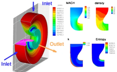
9.3 The Outlet Mass Flow Example

The developed software with presented boundary condi-tions was used for the simulation of the compressible

tur-bulent ﬂow in the 3D axis-symmetrical channel. Axisxis

the axis of symmetry. Example is shown in ﬁgure 11. At the inlet we used the boundary condition shown in section 6, conserving the total pressure, total temperature, and zero

tangential velocity, withθo =273.15 K ,po =101325 Pa.

The boundary condition shown in section 8 was used at

the outlet, with the given massﬂowG = 4.0 kg·s−1·m−2.

At each face, the value G was computed (in each

iter-ation) in order to match the massﬂow across the whole

boundary. The boundary condition preﬀering the zero

nor-mal velocity was used in the case of the inviscid flow. For the viscous turbulent flow, this condition was modi-fied by the zero velocity at the wall, and wall temperature

θW ALL =273.15 K was set. FurtherkW ALL =0 m2·s−2and

ωW ALL=cω_βy6μ2

s, cω 6

β =120.Here byyswe mean the

dis-tance between the face and the center of the neighbouring element.

Fig. 11.3D axis-symmetrical turbulent ﬂow, 3D geometry shape, results at chosen 2D crosscuts.

Another example demonstrates the capabilities of the new boundary condition in the use with the unstationary

(11)

Fig. 12.3D axis-symmetrical turbulent ﬂow, density isolines and velocity proﬁle at the outlet, 2D crosscut.

crosscut shown at ﬁgure 13, the inlet is located at the left

part of the boundary, the outlet points away from axis x.

Inlet boundary condition with the preference of total

quan-tities was used at the inlet,θo=875.00 K,po=101905 Pa.

The mass ﬂowG =0.75kg·s−1_·_m−2 _{was preferred at the}

outlet (in average). Wall temperature was set toθW ALL =

875.00 K. The computational mesh in 2D crosscut

con-sisted of 89x87 quadrilaterals.

Fig. 13.3D axis-symmetrical turbulent ﬂow, 3D geometry shape, results at chosen 2D crosscuts.

Conclusion

This paper is focused on the boundary conditions for 3D compressible ﬂow, and summarizes the work presented in [2], [8], [5], [6], [7], and other publications. The algorithms for the construction of 3D boundary conditions are pre-sented. The work is based on the analysis of the Riemann Problem for the split Euler equations and the modiﬁcations of this problem. Here the left hand side initial condition is replaced by various complementary conditions. The solu-tion of such problems is shown.

Acknowledgment

The results originated with the support of Ministry of the Interior of the Czech Republic, project SCENT, Grant MSM 0001066902 of the Ministry of Education of the Czech Re-public, and Ministry of Industry and Trade of the Czech Republic for the long-term strategic developmentof the re-search organization. The authors acknowledge this sup-port.