1
Improving Sea Level Anomaly Precision from Satellite Altimetry Using Parameters Correction in the Red Sea
Ahmed Mohammed Taqi1,2, Abdullah Mohammed Al-Subhi1 , Mohammed Ali Alsaafani1
1 Department of Marine Physics, King Abdulaziz University, Jeddah, Saudi Arabia 2Department of Marine Physics, Hodeihah University, Hodeihah, Yemen
Correspondence: Ahmed Mohammed Taqi ([email protected])
Abstract
An improved FSM method is used in geophysical and environmental corrections to enhance the final product of the along track Jason-2 SLA data and extend it near the Red Sea borders. In this study the ionospheric correction range, wet tropospheric correction range, sea state bias correction range and dry tropospheric correction range are enhanced and improved using FSM01, which helped to retrieve three more tracks (106, 170 and 234), earlier neglected by the distribution centers, and extend the tracks towards the coast. The FSM01 SLA is compared with Jason-2 SLA and AVISO SLA for the available 5 tracks, in which the FSM01 SLA show a good agreement and higher correlation with the Jason-2 SLA compared with that of AVISO, in addition to that it fills the gaps in the times series of all tracks. The new retrieved tracks also compared with those retrieved by AVISO, both data show similar variability, with FSM01 SLA show no gaps in the time series. The FSM01 SLA also extended towards the coast and show high correlation with the coastal tide measurements.
Introduction
The sea surface topography has been measured using satellite altimetry from space for more than three decades. These altimeteric measurements are considered a cornerstone any monitoring system in oceans; since they are used extensively to comprehend the ocean dynamics such as ocean observation and prediction models and management of climate change consequences (Chelton et al., 2001; Le Traon, 2013). Therefore, these products are most directly affected by the quality and availability at the appropriate times of altimeter data (Le Traon, 2011).
Since the late 1980s, several altimetry projects have been started. The open ocean radar and data processing tools have been improved, while sea level observation face some difficulties in coastal areas, leads to deterioration in data accuracy near the coast about 30 to 50 km ( Birol and Delebecque, 2014; Gommenginger et al., 2011; Anzenhofer et al., 1999). This is due to the complex conditions faced by coastal areas, including their closeness to the land and the effect of the costal bottom topography and water dynamics, which cause a difficulty in extracting information usable directly from the waveform Additional difficulties and challenges for measuring sea surface height using satellite altimetry near the coasts such as the radar echo which
2
affected by land surroundings and the inland water surface reflection. these difficulties complicated the interpretation of the signal within the coast borders that extends 5 to 10 km (Deng and Featherstone, 2006; Hwang et al., 2006; Gommenginger et al.,2011). The second challenge is geophysical and environmental corrections in the coastal areas is not as good as in the open ocean (e.g. dry troposphere, ionosphere, sea state bias, wave height, high-frequency wind effect, and tides) (Andersen and Scharroo, 2011). During the distribution of the data, the satellite operations centers usually remove the SLA data within about 50 km from the coast. Additionally, because of the low capture upon a wide range of near the coastal, satellite altimetry faces difficulty with the place and time of sampling (Birol et al., 2010).
However, the coastal ocean observation is extremely important: the coastal ocean considered as a region of most biological production and economic areas are directly influenced by the activity of human. Moreover, climate change can likely exacerbate many problems faced by coastal environments: coastal erosion, the flood of the coastal area, water pollution, exertion and damage to coastal biodiversity (Harley et al., 2006). To achieve this goal, altimetry data must be improved in shallow waters (Vignudelli et al., 2011). In the last decades, there were excellent enhancements have been made for the data processing and algorithms ( Passaro et al., 2014; Vignudelli et al., 2011)..One of the important improvements for coastal altimetry data was conducted through the French-Italian project ALBICOCCA (ALtimeter-Based Investigations in COrsica, Capraia, and Contiguous Areas). One of its resulting products was the establishment of data for the northwestern Mediterranean at the coast by (Vignudelli et al., 2006). Another study used T/P data with in-situ current data as well as tidal measurements in on the Corsica channels. Several other studies have dealt with the constraints on coastal altimetry, possible improvements in recent years, including ( Ghosh et al., 2015; Hwang et al., 2006; Deng and Featherstone, 2006; Deng et al., 2002; Brooks et al., 1998)
These improvements have given considerable momentum where AVISO launched two major projects dedicated to the advancement of coastal altimetry products for specific assignment: PISTACH, funded by the French Space Agency (CNES) for the processing of the coastal heights of Jason-1 and Jason-2 (Mercier et al., 2008); COASTALT (www.coastalt.eu), funded by the European Space Agency (ESA) for the design and implementation of a model for coastal regions altimetry processing for Envisat. In addition to that, NASA has also made their own coastal regions altimetry research through specific R&D project in reply to the finally OSTST call in 2008.
Recent developments in improving corrections and data processing in coastal zones, make it possible to increase data quality and quantity (Cipollini et al., 2008). For example, the study on the coasts of the Northwest Mediterranean in some T/P tracks. which improve data near coastal and in the open sea compared the AVISO products
3
The Red Sea is a narrow body of seawater separating the African and Asian continents. It is oriented north and northwest between 12° to 30° N with about 2300 km long and 280 km wide on average. The main connect to the Gulf of Aden and Indian Ocean is via the Strait of Bab el Mandeb from the south and in the north divided into two narrow Gulfs; Gulf of Suez and the Gulf of Aqaba while connecting the Mediterranean Sea through the Suez Canal. The marine environment in the Red Sea plays an important economic role, with abundant mineral resources including oil and gas. The Sea influences the country's strategy which has special importance in maritime transport. In most cases, the marginal sea (semi-enclosed basin) plays an important role in the world's navigation routes, maritime transport, and connecting countries.
The lack of sea-level data is the main constraint for the analysis of sea-level changes in coastal areas, especially for the Red Sea. There are no previous studies using satellite SLA near the coast in the Red Sea except (Taqi et al., 2017; Taqi et al. 2019). They extrapolate the Jason-2 SLA level3 data towards the coast by applying the FSM model to the SLA data only for the available level3 Jason-2 tracks. Unfortunately, due to the narrow width of the Red Sea, the operation centers remove unreliable data prior to level 3 product distribution and hence; some tracks are neglected in the Red Sea (for example; tracks 106, 170 and 234). Therefore, the main aim of this study is to use level 0 Jason-2 data to recover the neglected tracks and improve the accuracy of the SLA data in entire Red Sea. In this study, the Fourier Series model (introduced by (Taqi, et, al. 2017)), is used on range corrections to improve the final production of SLA data for Jason-2 tracks and enhance SLA data near the coast. Not only that, but it helps retrieving the neglected tracks by distributing centers. T The following sections of this paper are as follow: material and methods in the second section, the third section represent results and discussions and the final section for conclusion.
Material and Methods
Data
The satellite altimetry data used in this study is from Jason-2 along-tracks (level_0) in a weekly time span from June 2009 (cycle 33) to December 2014 (cycle 239). Those data are available through the JPL Physical Oceanography Distribution Active Archive center (ftp://podaac. jpl.nasa.gov/allData/ostm/preview/L2/GPS-OGDR/).
The Archiving Validation and Interpretation of Satellite Oceanographic (AVISO) downloaded from (ftp://ftp.AVISO.oceanobs.com/pub/oceano/AVISO/SSH/duacs/Data_Test/global/delayed-time/ along-track/). The four tide gauge stations used for the validation of the FSM01 SLA data obtained from the General Commission of Survey (SGS) in the Kingdom of Saudi Arabia and details are showed in Table (1).
For studies of sea surface variations, it is more appropriate to refer to the sea surface height to average sea level height, so-called sea level anomaly hsla, as the following equation;
4
Where (H) the satellite orbit above the reference ellipsoid, R is corrections for the different components (Range Robs), dry tropospheric correction (Rdry), wet tropospheric correction (Rwet),
ionospheric correction (Riono), sea state bias (Rssb)),dynamic atmosphere correction (hatm), tide
correction (htid), geoid correction (hgeo)). Robs = ct/2, R is the calculated range of travel time (t)
observed by the onboard ultra-stable oscillator (USO), and c is the velocity of the radar pulse that ignores refraction.
Methods
Several studies have been devoted to assess and improve some of the altimeter corrections in costal oceanographic environments (Andersen and Scharroo, 2011; Obligis et al., 2011; Ray et al., 2011; Fernandes et al., 2015, Taqi et al 2017). However, a very few studies included analyses of the various corrective terms as an entire, with the aim to increase the number of coastal SLA data to the end-users.
In this study, an improved FSM method is used to correct the parameter correction rangefor production SLA data for all tracks in the level0 Jason-2 in the Red Sea, as follows
The first step is to use mean and standard deviation to remove the anomalous from the correction data to produce SLA form the Eq. (2).
Correction< =mean±3σ (2)
The second step is to reconstruction the correction using the Fourier series equation along the track using Eq. (3) (Bloomfield 2000; Thomson and Emery 2014).
Fourier series Equation of correction
𝑚𝑚𝑠𝑠𝑠𝑠(𝑥𝑥)𝑓𝑓𝑓𝑓𝑓𝑓𝑓𝑓 =𝑠𝑠0+�(𝑠𝑠𝑖𝑖∗cos(𝑤𝑤 ∗ 𝑛𝑛 ∗ 𝑥𝑥)+𝑏𝑏𝑖𝑖sin( 𝐷𝐷
𝑖𝑖=1
𝑤𝑤 ∗ 𝑛𝑛 ∗ 𝑥𝑥) (3)
Where a is intercept, (ai and bi) represent the amplitude of the cosine and sine respectively, w shows the fundamental frequency of the signal, D is the number of degrees estimated in equation (4) following (Daniell 1946; Thomson and Emery 2014), and x is the distance between track points.
𝐷𝐷= 2𝑎𝑎𝑖𝑖 (4)
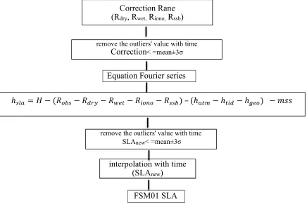
The third step is calculating the level-3 data by using equation (1). The fourth step is removing anomalous from SLA data by using filters of mean and standard deviation (3σ). In the final step, The linear interpolation has been applied to the SLA over time to create new data called FSM01, see the chart of each step of this method as shown in figure 1.
Table.1 The coastal tide gauge stations position and time period.
Name station Latitude Longitude Time
5
Jason-2 satellite tracks do not intersect with tide stations on the coast. Yanbu station is the closest station to the 132 and 246 tracks, the distance between the station and the track132 and track 246 is 4 and 6 kilometers respectively. The station data were used to compare the results of the FSM01 method and station data at the intersection of Jason-2 track with the coast by linear interpolation from Yanbu station.
Figure 1. Shows the Schematic streamline for the steps of the FSM01 method.
Result and Discussion
Despite the notable success of altimetry in the open ocean, which provides SLA data with high accuracy. However, in the coastal zones, the accuracy is degraded due to the surrounding terrain effects, combined with the lack of precision in some of the geophysical corrections and rapid changes in sea level. Several studies have been applied to assess and improve some altimeter corrections in coastal areas (Fernandes et al., 2015; Obligis et al., 2011; Vignudelli et al., 2011). In order to improve the accuracy and completeness of SLA data in Red Sea region derived from satellite altimetry, the FSM01 method was developed to improve geophysical and environmental corrections. Where it was able to improve the geophysical and environmental corrections along tracks for Jason-2 in the Red sea.
1- Ionospheric correction
FSM01 SLA Equation Fourier series
remove the outliers' value with time
SLAnew< =mean±3σ
interpolation with time (SLAnew)
Correction Rane (Rdry, Rwet, Riono, Rssb)
ℎ𝑠𝑠𝑠𝑠𝑠𝑠 =𝐻𝐻 −(𝑅𝑅𝑜𝑜𝑜𝑜𝑠𝑠− 𝑅𝑅𝑑𝑑𝑑𝑑𝑑𝑑− 𝑅𝑅𝑤𝑤𝑤𝑤𝑤𝑤− 𝑅𝑅𝑖𝑖𝑜𝑜𝑖𝑖𝑜𝑜− 𝑅𝑅𝑠𝑠𝑠𝑠𝑜𝑜) – (ℎ𝑠𝑠𝑤𝑤𝑎𝑎 − ℎ𝑤𝑤𝑖𝑖𝑑𝑑 − ℎ𝑔𝑔𝑤𝑤𝑜𝑜) − 𝑚𝑚𝑚𝑚𝑚𝑚
6
Ionospheric correction (Riono) is one the component used to estimate a sea-level from a satellite
altimeter. Where it is noisy and must be filtered spatially before removing it from the altimeter range. Figure 2a illustrates the original along-track record of cycle 116 of Jason-2 along the track 132 in the Red Sea, where the Riono was smoothed by using the FSM01 method. Fig 2b and C
exhibit the Hovmöller diagram of track 132 before and after Riono, respectively. it shown that the
FSM01 method helps increase and enhance the original along-track record of ionospheric corrections (IOC) as shown in Fig 2 especially near the coast.
Figure 2 The Riono for (A) the cycle 116 of Jason-2 along the track 132 in the Red Sea, before
(blue circles) and after (black line) and the Hovmöller diagram for the Riono data (B) original (C)
FSM01.
2- wet tropospheric correction
The wet tropospheric correction (Rwet) is the path delay correction due to cloud liquid water and
water vaper (Desportes et al, 2007). It is one of the major source for error of altimeter sea level in coastal areas (Andersen and Scharroo, 2011). he standard along-track register for Rwet. was include in
the FSM01 model. Figure 3a represents comparison between the original along-track data and the corrected Rwet. Where it illustrates that the corrected values are smoother than the original
along-A
C B
A
7
track Jason-2. Figure 3b, c showed the Hovmöller diagram for the original along-track record and the result of Rwet respectively. The FSM01 method was able to fill the gap in the data, which will
enhances producing SLA.
Figure 3 The cycle 116 of Jason-2 along the track 132 in the Red Sea, before (red circles) and after (blue line) the Rwet correction, the Hovmöller diagram for the Rwet data (B) original (c)
FSM01.
3- Sea state bias correction
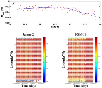
Sea State Bias (Rssb) is an altimeter ranging error due to the presence of ocean waves on the
surface. The rapidly changing properties of wind and waves which form a noise waveform that cause a major problem facing coastal altimetry.. Figure (4a) illustrate cycle 116 of Jason-2 along the track 132 in the Red Sea, the result of FSM01 is compared with the original. Figure 4b, c represents the Hovmöller diagram for the original and FSM01, where the FSM01 method was able to create new data more accurate than the original near the Red Sea coast.
B C
8
Figure 4 (A) The Sea state bias correction for the cycle 116 of Jason-2 along the track 132 in the Red Sea, before (red circles) and after (blue line) and the Hovmöller diagram for the Rssb data (B)
original (C) FSM01.
4- Dry tropospheric correction (Rdry)
Dry tropospheric correction (Rdry) depends on the dry gas component of the atmosphere. It is by
far the largest adjustment range in satellite altimetry. With magnitude about 2.3 m at sea level and a range of about 0.2 m (Fernandes et al., 2014), its temporal variation is low. Dry tropospheric range depend on the sea level pressure and latitude. FSM01 method was used in dry tropospheric correction to enhance accuracy near the coast. Figure 5(a, b, and c) show FSM01 corrected Rdry
matched with the original data. FSM01 enhanced Rdry data near the coast (As seen in the
9
Figure 5 (A) The Rdry for the cycle 116 of Jason-2 along the track 132 in the Red Sea, before (red
circles) and after (blue line) and the Hovmöller diagram for the Rdry data (B) original (c) FSM01.
5- SLA quality inferred from FSM01
The accuracy of the altimeter SLA depends on many of the corrections used to produce sea level, namely, geophysical and environmental corrections. The FSM01 method was used on the geophysical and environmental corrections, which required for the estimation of the Jason-2 SLA data. The method allows to enhance and improve the correction ranges, which in turn helped to retrieve new tracks, which earlier neglected by the distribution centers and extend the SLA data to the coast. In this section, the SLA from the FSM01 method is compared with the Jason-2 SLA and AVISO SLA for the period 2009-2014 for available 5 tracks (Figure 6). The times series of the five available tracks show that FSM01 SLA agreed will with Jason2 SLA variability and also fill the gaps within the times series more than AVISO SLA do as shown in fig (6).
10
Figure 6. Time series of SLA for closest point of the tracks to the coast for Jeson2 (black), with FSM01 SLA (Red) and AVISO (blue).
11
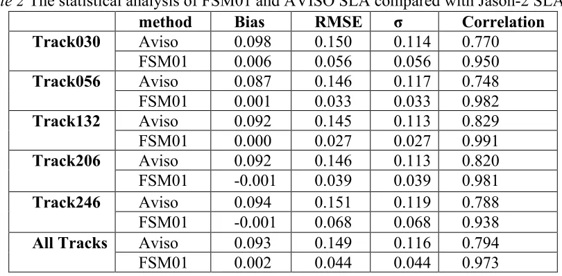
Jason-2 with correlation coefficient 0.973. The scatter index for FSM01 is almost 0.3 m as compared with that of AVISO (0.83 m).
Table 2 The statistical analysis of FSM01 and AVISO SLA compared with Jason-2 SLA
method Bias RMSE σ Correlation
Track030 Aviso 0.098 0.150 0.114 0.770
FSM01 0.006 0.056 0.056 0.950
Track056 Aviso 0.087 0.146 0.117 0.748
FSM01 0.001 0.033 0.033 0.982
Track132 Aviso 0.092 0.145 0.113 0.829
FSM01 0.000 0.027 0.027 0.991
Track206 Aviso 0.092 0.146 0.113 0.820
FSM01 -0.001 0.039 0.039 0.981
Track246 Aviso 0.094 0.151 0.119 0.788
FSM01 -0.001 0.068 0.068 0.938
All Tracks Aviso 0.093 0.149 0.116 0.794
FSM01 0.002 0.044 0.044 0.973
Figure 7 shows the density scatter diagram for the five tracks between FSM01 and AVISO with Jason-2. There is a clear fit between FSM01 SLA and Jason-2 SLA with a slope close to unity. While that of AVISO SLA with Jason-2 SLA deviated from to unity.
The addition advantage of this study is the retravel of the neglected tracks by the final Jason-2 level 3 product (tracks 106,170, and 234). Even though AVISO product reproduces those tracks, with a good accuracy for open sea as seen, it still contains a lot of gaps in the coastal area FSM01 show better agreement with the coastal stations SLA.
12
Figure 7 the scatter distribution Comparison between SLA Jason-2 with FSM01 and AVISO for five tracks
Sea Level Anomaly (Track246)
Sea Level Anomaly (Track208) Sea Level Anomaly (Track132)
13
Figure 8 Comparison of the all tracks FSM01 SLA (Red) and AVISO (blue).
14
Table 4 The statistics of the FSM01 data with observation in the coastal region
Figure 9 comparing the coastal station SLA and interpolated SLA with the FSM01 SLA at the intersect with the coast.
Figure 10 a and b show the Hovmöller diagram of SLA along track 132 for Jason2 and FSM01. It is clear from the figure that, the FSM01 is able to fill the gaps in the time series and extend the SLA towards both coasts of the Red Sea.
Bias RMSE std Correlation
Track030 0.07 0.10 0.07 0.92
Track056 0.09 0.14 0.10 0.84
Track132 0.02 0.08 0.08 0.92
Track206 0.14 0.19 0.13 0.80
15
Figure 10: The Hovmöller diagram of SLA along track 132 for (a) Jason2 and (b) FSM01 from cycle 33 to cycle 239
conclusion
Generally, in this study, the FSM01 method was used in geophysical and environmental corrections for enhancing SLA Jason-2 along tracks data and extend it near the coast of the Red Sea. This study improves the SLA data along the Satellite tracks using enhanced and improved ionospheric correction range, wet tropospheric correction range, sea state bias correction range and dry tropospheric correction range by FSM01 method. The FSM01 method is reliable in detection of anomalous values in satellite altimeter corrections and better reconstruction of lost or rejected values. The FSM01 SLA show high correlation with Jason-2 SLA for the available 5 tracks as compared with that of AVISO SLA. In addition to that, it fills the gaps in the times series of the tracks. This method has retrieved three additional tracks (106, 170 and 234), earlier neglected by the distribution centers. Even that those tracks were retrieved by AVISO, the new retrieved data by FSM01 show no gaps in the time series. This study found that FSM01 method is efficient in extending data to the coast, which show high correlation with the coastal tide gauge data.
Acknowledgment
16 References
Andersen, O.B., Scharroo, R., 2011. Range and geophysical corrections in coastal regions: and implications for mean sea surface determination, in: Coastal Altimetry. Springer, pp. 103– 145.
Anzenhofer, M., Shum, C.K., Rentsh, M., 1999. Coastal altimetry and applications. Ohio State Univ. Geod. Sci. Surv. Tech. Rep 464, 36.
Birol, F., Cancet, M., Estournel, C., 2010. Aspects of the seasonal variability of the Northern Current ( NW Mediterranean Sea ) observed by altimetry. J. Mar. Syst. 81, 297–311. doi:10.1016/j.jmarsys.2010.01.005
Birol, F., Delebecque, C., 2014. Journal of Marine Systems Using high sampling rate ( 10 / 20 Hz ) altimeter data for the observation of coastal surface currents : A case study over the
northwestern Mediterranean Sea. J. Mar. Syst. 129, 318–333. doi:10.1016/j.jmarsys.2013.07.009
Birol, F., Fuller, N., Lyard, F., Cancet, M., Nin, F., 2017. Coastal applications from nadir altimetry: Example of the X-TRACK regional products 59, 936–953. doi:10.1016/j.asr.2016.11.005 Brooks, R.L., Lockwood, D.W., Lee, J.E., Handcock, D., Hayne, G.S., 1998. Land effects on
TOPEX radar altimeter measurements in Pacific Rim coastal zones. Remote Sens. Pacific by Satell. 175–198.
Chelton, U.B., Ries, J.C., Haines, B.J., FU, L.-L., Callahan, P.S., 2001. Satellite Altimetry and Earth Sciences, in: FU, L.-L., Cazenave, A. (Eds.), Satellite Altimetry and Earth Sciences A Handbook of Techniques and Applications. Academic Press,A Harcourt Science and Technology Company, San Diego, California ,usa, pp. 1–122.
Cipollini, P., Gomez-Enri, J., Gommenginger, C., Martin-Puig, C., Vignudelli, S., Woodworth, P., Benveniste, J., 2008. Developing radar altimetry in the oceanic coastal zone: the COASTALT project. EGU Gen. Assem.
Deng, X., Featherstone, W.E., 2006. A coastal retracking system for satellite radar altimeter
waveforms : Application to ERS-2 around Australia. J. Geophys. Res. 111, 1–16. doi:10.1029/2005JC003039
Deng, X., Featherstone, W.E., Hwang, C., Shum, C.K., 2002. Improved Coastal Marine Gravity Anomalies at the Taiwan Strait from Altimeter Waveform Retracking 1–9.
Fernandes, M.J., Lázaro, C., Ablain, M., Pires, N., 2015a. Remote Sensing of Environment Improved wet path delays for all ESA and reference altimetric missions. Remote Sens. Environ. 169, 50–74. doi:10.1016/j.rse.2015.07.023
Fernandes, M.J., Lázaro, C., Ablain, M., Pires, N., 2015b. Improved wet path delays for all ESA and reference altimetric missions. Remote Sens. Environ. 169, 50–74. doi:10.1016/j.rse.2015.07.023
Fernandes, M.J., Lázaro, C., Nunes, A.L., Scharroo, R., 2014. Atmospheric Corrections for Altimetry Studies over Inland Water. Remote Sens. 4952–4997. doi:10.3390/rs6064952 Gaspar, P., Ogor, F., Le Traon, P., Zanife, O., 1994. Estimating the sea state bias of the TOPEX
and POSEIDON altimeters from crossover differences. J. Geophys. Res. Ocean. 99, 24981– 24994.
Ghosh, S., Kumar Thakur, P., Garg, V., Nandy, S., Aggarwal, S., Saha, S.K., Sharma, R., Bhattacharyya, S., 2015. SARAL/AltiKa Waveform Analysis to Monitor Inland Water Levels: A Case Study of Maithon Reservoir, Jharkhand, India. Mar. Geod. 38, 597–613. doi:10.1080/01490419.2015.1039680
17
Challenor, P., Gao, Y., 2011. Retracking altimeter waveforms near the coasts, in: Coastal Altimetry. Springer, pp. 61–101.
Guo, J., Chang, X., Gao, Y., Sun, J., Hwang, C., 2009. Lake level variations monitored with satellite altimetry waveform retracking. IEEE J. Sel. Top. Appl. Earth Obs. Remote Sens. 2, 80–86. doi:10.1109/JSTARS.2009.2021673
Guo, J.Y., Gao, Y.G., Hwang, C.W., Sun, J.L., 2010. A multi-subwaveform parametric retracker of the radar satellite altimetric waveform and recovery of gravity anomalies over coastal oceans. Sci. China Earth Sci. 53, 610–616. doi:10.1007/s11430-009-0171-3
Guo, Z., Cao, A., Lv, X., 2012. Inverse Estimation of Open Boundary Conditions in the Bohai Sea. Math. Probl. Eng. 2012, 1–10. doi:10.1155/2012/628061
Harley, C.D.G., Hughes, A.R., Hultgren, K.M., Miner, B.G., Sorte, C.J.B., Thornber, C.S., Rodriguez, L.F., Tomanek, L., Williams, S.L., 2006. The impacts of climate change in coastal marine systems. Ecol. Lett. 9, 228–241. doi:10.1111/j.1461-0248.2005.00871.x
Hwang, C., Guo, J., Deng, X., Hsu, H.Y., Liu, Y., 2006. Coastal gravity anomalies from retracked Geosat/GM altimetry: Improvement, limitation and the role of airborne gravity data. J. Geod. 80, 204–216. doi:10.1007/s00190-006-0052-x
Hwang, C., Hsu, H.-Y., Deng, X., 2003. Marine gravity anomaly from satellite altimetry: A comparison of methods over shallow waters, in: Satellite Altimetry for Geodesy, Geophysics and Oceanography. Springer, pp. 59–66.
Imel, D.A., 1994. Evaluation of the TOPEX/POSEIDON dual‐frequency ionosphere correction. J.
Geophys. Res. Ocean. 99, 24895–24906.
Khaki, M., Forootan, E., Sharifi, M.A., 2014. radar altimetry waveform retracking over the Caspian Sea. Int. J. Remote Sens. 35, 37–41. doi:10.1080/01431161.2014.951741
Langodan, S., Cavaleri, L., Viswanadhapalli, Y., Hoteit, I., 2015. Wind-wave source functions in opposing seas. J. Geophys. Res. Ocean. 120, 6751–6768. doi:10.1002/2015JC010816
Le Traon, P.Y., 2013. From satellite altimetry to Argo and operational oceanography: Three revolutions in oceanography. Ocean Sci. 9, 901–915. doi:10.5194/os-9-901-2013
Lekien, F., Coulliette, C., Bank, R., Marsden, J., 2004. Open-boundary modal analysis :
Interpolation , extrapolation , and filtering. J. Geophys. Res. 109, 1–13. doi:10.1029/2004JC002323
Obligis, E., Desportes, C., Eymard, L., Fernandes, M.J., Lázaro, C., Nunes, A.L., 2011. Tropospheric Corrections for Coastal Altimetry, in: Vignudelli, S., Kostianoy, A.G., Cipollini, P., Benveniste, J. (Eds.), Coastal Altimetry. Springer-Verlag Berlin Heidelberg, pp. 1–565. doi:10.1007/978-3-642-12796-0
Obligis, E, Desportes, C., Eymard, L., Fernandes, M.J., Nunes, A.L., Contamination, B.T., Configuration, I., 2011. Tropospheric Corrections for Coastal Altimetry. doi:10.1007/978-3-642-12796-0
Passaro, M., Cipollini, P., Vignudelli, S., Quartly, G.D., Snaith, H.M., 2014. ALES: A multi-mission adaptive subwaveform retracker for coastal and open ocean altimetry. Remote Sens. Environ. 145, 173–189. doi:10.1016/j.rse.2014.02.008
Rasul, N.M.A., Stewart, I.C.F., Nawab, Z.A., 2015. Introduction to the Red Sea: its origin, structure, and environment, in: The Red Sea. Springer, pp. 1–28.
18 doi:10.1007/978-3-642-12796-0_9
Taqi, A.M., Al-Subhi, A.M., Alsaafani, M.A., 2017. Extension of Satellite Altimetry Jason-2 Sea Level Anomalies Towards the Red Sea Coast Using Polynomial Harmonic Techniques. Mar. Geod. doi:10.1080/01490419.2017.1333549
Verron, J., Sengenes, P., Lambin, J., Noubel, J., Steunou, N., Guillot, A., Picot, N., Coutin-Faye, S., Sharma, R., Gairola, R.M., Raghava Murthy, D.V. a, Richman, J.G., Griffin, D., Pascual, A., Rémy, F., Gupta, P.K., 2015. The SARAL/AltiKa Altimetry Satellite Mission. Mar. Geod. 0419, 00–00. doi:10.1080/01490419.2014.1000471