Lower Bounds for Differentially Private RAMs

Lower Bounds for Differentially Private RAMs

Giuseppe Persiano1,2 _{and Kevin Yeo}1

1

Google LLC, Mountain View, [email protected] 2 _{Universit`a di Salerno, Salerno, Italy[email protected]}

Abstract. In this work, we study privacy-preserving storage primitives that are suitable for use in data analysis on outsourced databases within the differential privacy framework. The goal in differentially private data analysis is to disclose global properties of a group without compromis-ing any individual’s privacy. Typically, differentially private adversaries only ever learn global properties. For the case of outsourced databases, the adversary also views the patterns of access to data. Oblivious RAM (ORAM) can be used to hide access patterns but ORAM might be ex-cessive as in some settings it could be sufficient to be compatible with differential privacy and only protect the privacy of individual accesses. We consider (, δ)-Differentially Private RAM, a weakening of ORAM that only protects individual operations and seems better suited for use in data analysis on outsourced databases. As differentially private RAM has weaker security than ORAM, there is hope that we can bypass the

Ω(log(n/c)) bandwidth lower bounds for ORAM by Larsen and Nielsen [CRYPTO ’18] for storing an array ofnentries and a client withcbits of memory. We answer in the negative and present anΩ(log(n/c)) band-width lower bound for privacy budgets of=O(1) andδ≤1/3. Theinformation transfertechnique used for ORAM lower bounds does not seem adaptable for use with the weaker security guarantees of dif-ferential privacy. Instead, we prove our lower bounds by adapting the

chronogramtechnique to our setting. To our knowledge, this is the first work that uses the chronogram technique for lower bounds on privacy-preserving storage primitives.

1

Introduction

The traditional way to define the privacy of access pattern isobliviousness. An oblivious storage primitive ensures that any adversary that is given two sequences of operations of equal length and observes the patterns of data access performed by one of the two sequences cannot determine which of the two sequences induced the observed access pattern. The most famous oblivious storage primitive is Oblivious RAM (ORAM) that outsources the storage of an array and allows clients to retrieve and update array entries. ORAM was first introduced by Goldreich [15] who presented an ORAM with sublinear amortized bandwidth per operation for clients with constant size memory. Goldreich and Ostrovsky [16] give the first ORAM construction with polylogarithmic amortized bandwidth per operation. In the past decade, ORAM has been the subject of extensive research [27, 17, 30, 18, 20, 31, 26] as well as variants such as statistically secure ORAMs [7, 6], parallel ORAMs [1, 5, 4] and garbled RAMs [14, 13, 24]. The above references are just a small subset of all the results for ORAM constructions.

Instead, we focus on a different definition of privacy using differential pri-vacy [10, 9, 11]. The representative scenario for differential privacy is privacy-preserving data analysis which considers the problem of disclosing properties about an entire database while maintaining the privacy of individual database records. A mechanism or algorithm is considered differentially private if any fixed disclosure is almost as likely to be outputted for two different input databases that only differ in exactly one record. As a result, an adversary that views the disclosure is unable to determine whether an individual record was part of the input used to compute the disclosure. We consider the scenario of performing privacy-preserving data analysis on data outsourced to an untrusted server. By viewing the patterns of access to the outsourced data, the adversarial server might be able to determine which individual records were used to compute the disclosure compromising differential privacy.

One way to protect the patterns of data access is to outsource the data using an ORAM. However, in many cases, it turns out that the obliviousness guaran-tees of ORAM may be stronger than required. For example, let’s suppose that we wish to disclose a differentially private regression model over a sample of the outsourced data. ORAM guarantees that the identity of all sampled database records will remain hidden from the adversary. On the other hand, the differen-tially private regression model only provides privacy about whether an individual record was sampled or not. Instead of obliviousness, we want a weaker notion of privacy for access patterns suitable for use with differentially private data analytics. With a weaker notion of privacy, there is hope for a construction with better efficiency than ORAM.

stor-age primitive that outsources the storstor-age of an array in a manner that allows a client to retrieve and update array entries while providing differentially pri-vate access. As this privacy notion is weaker than obliviousness, theΩ(log(n/c)) lower bounds for ORAMs that store n array entries and clients with c bits of storage by Larsen and Nielsen [22] do not apply. There is hope to achieve a dif-ferentially private RAM construction with smaller bandwidth. In this work, we answer in the negative and show that an Ω(log(n/c)) bandwidth lower bound also exists for differentially private RAM for typical privacy budgets of=O(1) and δ ≤ 1/3. As differential privacy with budgets of = O(1) and δ ≤ 1/3 provide weaker security than obliviousness, any ORAM is also a differentially private RAM. Therefore, our lower bounds show that the ORAM construction by Patel et al. [26] is an asymptotically optimal, up to an O(log logn) factor, differentially private RAM with=O(1) andδ≤1/3.

1.1 Our Results

In this section, we will present our contributions. We first describe the scenarios where our lower bounds apply. Our lower bounds apply todifferentially private

RAMs that process operations in an online fashion. The RAM must be both

read-and-write, that is, the set of permitted operations include both reading and writing array entries. The server that stores the array is assumed to be

passive in that the server may not perform any computation beyond retrieving and overwriting cells but no assumptions are made on the storage encoding of the array. Finally, we assume that the adversary iscomputationally bounded. We now go into detail about each of these requirements.

Differential Privacy. The goal of differential privacy is to ensure that the removal or replacement of an individual in a large population does not significantly affect the view of the adversary. Differential privacy is parameterized by two values 0 ≤, δ ≤1. The value is typically referred to as the privacy budget. When δ= 0, the notion is known aspuredifferential privacy while, ifδ >0, the notion is known as approximate differential privacy. In our context, an individual is a single operation in a sequence (thepopulation) of read (also called queries) and write (also called updates) operations over an array of n entries stored on a, potentially adversarial, remote server. For any implementationDSand for any sequence Q, we define VDS(Q) to be the view of the server when sequence Q is executed byDS. A differentially private RAM,DS, is defined to ensure that the adversary’s view on one sequence of operations should not be significantly different whenDSexecutes another sequence of operations which differs for only one operation. We assume that our adversaries are computationally bounded.

Formally, ifDSis (, δ)-differentially private, then for any two sequencesQ1 and Q2 that differ in exactly one operation, it must be that Pr[A(VDS(Q1)) = 1]≤e_Pr[A(

in [25]. In the majority of scenarios, differential privacy is only considered use-ful for the cases when=O(1) and δis negligible. This is exactly the scenario where our lower bounds will hold. In fact, our lower bounds hold for anyδ≤1/3. We note that differential privacy with =O(1) andδ ≤1/3 is a weaker secu-rity notion than obliviousness. Obliviousness is equivalent to differential privacy when= 0 andδis negligible. Therefore, our lower bounds also hold for ORAM and match the lower bounds of Larsen and Nielsen [22]. We refer the reader to Section 2 for a formal definition of differential privacy.

Online RAMs. It is important that we discuss the notion of onlinevs. offline

processing of operations by RAMs. In the offline scenario, it is assumed that all operations are given before the RAM must start processing updates and an-swering queries. The first ORAM lower bound by Goldreich and Ostrovsky [16] considered offline ORAMs with “balls-and-bins” encoding and security against an all-powerful adversary. “Balls-and-bins” refers to the encoding where array entries are immutable balls and the only valid operation is to move array entries into various memory locations referred to as bins. Boyle and Naor [2] show that proving an offline ORAM lower bound for non-restricted encodings is equivalent to showing lower bounds in sorting circuits, which is a long-standing problem in complexity. Instead, we consider online RAMs where operations arrive one at a time and must be processed before receiving the next operation. The as-sumption of online operations is realistic as the majority of RAM constructions consider online operations and almost all applications of RAMs consider online operations. Our lower bounds only apply for online differentially private RAMs.

Read-and-Write RAMs. Traditionally, all ORAM results consider the scenario where the set of valid operations include both reading and writing array entries. A natural relaxation would be to considerread-onlyRAMs where the only valid operation is reading array entries. Any lower bound on read-only RAMs would also apply to read-and-write RAMs. However, in a recent work by Weiss and Wichs [35], it is shown that any lower bounds for read-only ORAMs would imply very strong lower bounds for either sorting circuits and/or locally decodable codes (LDCs). Proving lower bounds for LDCs has, like sorting circuits, been an open problem in the world of complexity theory for more than a decade. As differential privacy is weaker than obliviousness, any lower bounds on read-only, differentially private RAMs also imply lower bounds on read-only ORAMs. To get around these obstacles, our work focuses only on proving lower bounds for read-and-write differentially private RAMs.

Passive Server. In our work, we will assume that the server storing the array is

on computation, we can reinterpret our results as lower bounds on the amount of server computation required.

We now informally present our main contribution.

Theorem 1 (informal).LetDSbe any online, read-and-write RAM that stores

narray entries each of sizebbits on a passive server without any restrictions on storage encodings. Suppose that the client hascbits of storage. Assume thatDS

provides (, δ)-differential privacy against a computational adversary that views all cell probes performed by the server. If =O(1) and 0 ≤δ ≤1/3, then the expected amortized bandwidth of both reading and writing array entries by DS

isΩ(blog(n/c))bits or Ω(log(n/c))array entries. In the natural scenario where

c≤nαwhere 0≤α <1, thenΩ(logn)array entries of bandwidth are required.

We note that our lower bounds are tight up to anO(log logn) factor since PanORAMa [26] requires onlyO(lognlog logn) array entries of bandwidth when-everb=Ω(logn) and any ORAM is also a differentially private RAM with= 0 and negligible δ. Furthermore, whenb=Ω(log2n), Path ORAM [31] is tight.

1.2 Previous Works

In this section, we present a small survey of previous works on data structure lower bounds. We also describe the first lower bound for data structures that provide privacy guarantees.

The majority of data structure lower bounds are proved using the cell probe model introduced by Yao [36], which only charges for accessing memory and allows unlimited computation. In the case for passive servers that only retrieve and overwrite memory, the costs of the cell probe model directly imply costs in bandwidth. Thechronogramtechnique was introduced by Fredman and Saks [12] which can be used to proveΩ(logn/log logn) lower bounds. Pˇatra¸scu and De-maine [29] presented theinformation transfertechinque which could be used to prove Ω(logn) lower bounds. Larsen [21] presented an ˜Ω(log2n) lower bound for two-dimensional dynamic range counting, which remains the highest lower bound proven for any lognoutput data structures. Recently, Larsen et al.[23] presented an ˜Ω(log1.5n) lower bound for data structures with single bit outputs which is the highest lower bound for decision query data structures.

and Wichs [35] show that lower bounds for online, read-only ORAMs would imply lower bounds for either sorting circuits and/or locally decodable codes.

We present a brief overview of the techniques used by Larsen and Nielsen [22], which uses the information transfer technique. We also describe why information transfer does not seem to be of use for differentially private RAM lower bounds. Information transfer first builds a binary tree over Θ(n) operations where the first operation is assigned to the leftmost leaf, the second operation is assigned to the second leftmost leaf and so forth. Each cell probe is assigned to at most one node of the tree as follows. For a cell probe, we identify the operation that is performing the probe as well as the most recent operation that overwrote the cell that is being probed. The cell probe is assigned to the lowest common ancestor of the leaves associated with the most recent operation to overwrite the cell and the operation performing the probe. Let us fix any node of the tree and consider the subtree rooted at the fixed node. It can be shown that the probes assigned to the root is the entirety of information that can be transferred from the updates of the left subtree to be used to answer queries in right subtree. Consider the sequence of operations where all leaves in the left subtree write a randomly chosen b-bit string to unique array entries and all leaves in the right subtree read an unique, updated array entry. For any DS to return the correct b-bit strings asked by the queries in the right subtree, a large amount of information must be transferred from the left subtree to the right subtree. Thus, many probes should be assigned to the root of this subtree. Suppose that for another sequence of operations, DSassigns significantly less probes to the root of this subtree. Then, a computational adversary can count the probes and distinguish between the worst case sequence and any other sequence contradicting obliviousness. As a result, there must be many probes assigned to each node of the information transfer tree. Each cell probe is assigned to at most one node. So, summing up the tree provides a lower bound on the number of cell probes required.

1.3 Overview of our Proofs

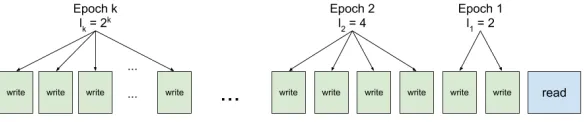
In this section, we present an overview of the proof techniques used in Sections 3 and 4. Our lower bounds use ideas from works by Pˇatra¸scu and Demaine [29] and Pˇatra¸scu [28]. However, we begin by reviewing the original chronogram technique of Fredman and Saks [12]. Let us suppose thattwis the running time of an update (write) and tr is the running time of a query (read). Consider a sequence of operations with Θ(n) updates followed by a single query. Starting from the query and going backwards in time, updates are partitioned into exponentially increasing epochs at some rate r. Epochs are indexed in reverse time, so the smallest epoch closest to the query is epoch 1. Thei-th epoch will have`i =ri update operations. The goal of the chronogram is to prove that there exists a query that requires information from many of the epochs simultaneously. To do this, we first observe that if each update writes a randomly and independently chosen b-bit entry, an update operation preceding epoch i cannot encode any information about epochi. Therefore, all information about epochican only be found in cells that have been written as part of the update operations of epoch i or any following epochs. Since each update stores b random bits, any epoch i encodes at least `i·b bits in total. If we denote by w the number of bits in a cell and set r= (tww)2, it is easy to see that the write operations of epochs i−1, i−2, . . . ,1 can probe at mosttw(ri−1+. . .+r) =O(`i/(tww2)) cells and write at mostO(`i/(tww)) bits. As a result, the majority of the bits encoded by updates in epoch i remain in cells last written in epoch i. Finally, the goal is to construct a random query such thatΩ(b) bits must be transferred from each epoch. If such a query exists, we can prove that max{tw, tr}=Ω((b/w) logrn) = Ω((b/w) logn/log logn).

This lower bound can be improved toΩ((b/w) logn) by using an improve-ment of the chronogram technique by Pˇatra¸scu [28]. In the original chronogram technique, the epochs are fixed since the query’s location and the number of updates are fixed. An algorithm may attempt to target an epoch i by having all future update operations encode information only about epoch i. To coun-teract this, we consider a harder update sequence where epoch locations cannot be predicted by the algorithm. Specifically, we consider a sequence that consists of a random number of update operations followed by a single query opera-tion. For such a sequence, even if an algorithm attempts to target epoch i, it cannot pinpoint the location of epoch i and may only prepare over all possi-ble query locations. We show that any update operation may now only encode O(tww/logrn) about epochiwhere logrnis the number of epochs. As a result, future update operations can only encode aO(1/log_rn) fraction as much infor-mation about epoch i as the previous lower bound attempt. This allows us to fixr= 2 which increases the number of epochs logn. If we can find a query that requires Ω(b) bits of information transfer from the majority of epochs, we can prove that max{tw, tr}=Ω((b/w) logn).

the updated array entry is chosen independently and uniformly at random from

{0,1}b<sub>. Focus on an epochi and consider picking a random query from the `</sub> i array indices updated in epochi. The majority of these queries must readΩ(b) bits from cells last written in epochias future operations cannot encode all`i·b bits encoded by epochi. As a result, there exists some query such thatΩ(b) bits must be transferred from epochifor all sufficiently large epochs. We use differ-ential privacy to show that Ω(b) bits must be transferred from all sufficiently large epochs. Consider two sequences of operations that only differ in the final query operation where one query requiresΩ(b) bits from epochifor correctness while the other query does not need any information from epochi. If the latter query transferso(b) bits from epochi, the adversary can distinguish between the two sequences with high probability contradicting differential privacy. Note, our privacy guarantees do not degrade significantly as the two sequences only differ at the final query operation. Therefore, we can prove that Ω(b) bits have to be transferred from most epochs and that max{tw, tr}=Ω((b/w) logn). The proof of this lower bound is found in Section 3.

A stronger lower bound is presented in Section 4 using more complex epoch constructions. We now describe our main result presented in Section 4. The lower bound outlined above shows that max{tw, tr}=Ω((b/w) logn) but does not preclude the case where tw =Θ((b/w) logn) and tr =O(1), for example. We show this cannot be the case. In particular, we show that if max{tw, tr}= O((b/w) logn), then it must be the case that tw = Θ((b/w) logn) and tr = Θ((b/w) logn). The idea is to construct different epoch constructions for the cases whentwandtr are small respectively. Whentw=o((b/w) logn), we know that operations in future epochs cannot encode too much information. We con-sider an epoch construction where epochs grow by a rate of r = ω(1) every r epochs increasing the number of epochs to ω(logn). In exchange, there are many operations after an epochi. Sincetw is small, the future operations may not encode too much information about epoch iensuring most of the informa-tion about epoch i remain in cells last written during epoch i. As a result, it can be shown again thatΩ(b) bits must be read from many epochs implying an tr=ω((b/w) logn) lower bound.

2

Differentially Private Cell Probe Model

We start by formalizing the model for which we prove our lower bounds. We rely on thecell probe model, first described by Yao [36], and typically used to prove lower bounds for data structures without any requirements for privacy of the stored data and/or the operations performed. In a recent work by Larsen and Nielsen [22], the oblivious cell probe modelwas introduced and used to prove a lower bound for oblivious RAM. The oblivious cell probe model was defined for any data structures where the patterns of access to memory should not reveal any information about the operations performed. We generalize the oblivious cell probe model and present the (, δ)-differentially private cell probe model. In this new model, all data structures are assumed to provide differential privacy for the operations performed with respect to memory accesses viewed by the adversary. The differentially private cell probe model is a generalization of the oblivious cell probe model as obliviousness is equivalent to differential privacy with = 0 and δ =negl(n), that is, any function negligible in the number of items stored in the data structure.

The cell probe model is an abstraction of the interaction between CPUs and word-RAM memory architectures. Memory is defined as an array of cells such that each cell contains exactlywbits. Anyoperationof a data structure is allowed to probecells where a probe can consist of either reading the contents of a cell or overwriting the contents of a cell. The running time or cost for any operation of a data structure is measured by the number of cell probes performed. An algorithm is free to do unlimited amounts of computation based on the contents of probed cells.

The cell probe model does not effectively capture the correct scenario for data structures that provide privacy of the operations performed such as obliv-ious RAM. The typical scenario considered involves two parties denoted the

client and the server. The client outsources the storage of data to the server while maintaining the ability to perform some set of operations over the data efficiently. In addition, the client wishes to hide the operations performed from the adversarial server that views the contents of all cells in memory as well as the sequence of cells probed in memory. We importantly note that the server does not learn about the contents and sequence of accesses to the client’s storage. For this reason, Larsen and Nielsen [22] defined the oblivious cell probe model to prove lower bounds for oblivious RAMs. We note that the differentially pri-vate cell probe model is identical to the oblivious cell probe model except for the simple replacement of obliviousness with differential privacy as the privacy requirement. For a full description of the oblivious cell probe model, we refer the reader to Section 2 of [22].

To define the differentially private cell probe model, we first describe adata structure problemas well as a differentially private cell probe data structurefor any data structure problem.

Definition 1. A data structure problem P is defined by a tuple (U, Q, O, f)

1. U is the universe of all update operations; 2. Qis the universe of all query operations;

3. O is domain of all possible outputs for all queries;

4. f :U∗_{×Q→O is a function that describes the desired output of any query} q∈Qgiven the history of all updates, (u1, u2, . . . , um)∈U∗.

A differentially private cell probe data structure DS for the data structure problemP consists of a randomized algorithm implementing update and query operations forP.DSis parameterized by the integerscandwdenoting the client storage and cell size in bits respectively. Additionally, DS is given a random stringRof finite lengthrcontaining all randomness thatDSwill use. Note that

R can be arbitrarily large and, thus, contain all the randomness of a random oracle. Given the random string, our algorithms can be viewed as deterministic. Each algorithm is viewed as a finite decision tree executed by the clientthat probes (read or overwrite) memory cells owned by the server. For each q∈ Q and u ∈ U, there exists a (possibly) different decision tree. Each node in the decision tree is labelled by an index indicating the location of the server-held memory cell to be probed. For convenience, we will assume that a probe may both read and overwrite cell contents. This only reduces the number of cell probes by a factor of at most 2. Additionally, all leaf nodes are labelled with an element ofO indicating the output ofDSafter execution.

Each edge in the tree is labelled by four bit strings. The first bit-string of length w represents the contents of the cell probed. The next w-bit string represents the new cell contents after overwriting. There are two c-bit strings representing the current client storage and the new client storage after perform-ing the probe. Finally, there is a r-bit string representing the random string. The client executes DS by traversing the decision tree starting from the root. At each node, the client reads the indicated cell’s contents. Using the random string, the current client storage and the cell contents, it finds the edge to the next node and updates the probed cell’s contents and client storage accordingly. When reaching a leaf, DSoutputs the element ofO denoted at the leaf.

Note,DSis only permitted to use the contents of the previously probed cell, current client storage and the random string as input to generate the next cell probe or produce an output. The running time of DS is related to the depth of the decision tree as each edge corresponds to a cell probe. Furthermore, as the servers are passive, the server can only either update or retrieve a cell for the client. As a result, the running time (number of cell probes) multiplied by w(the cell size) gives us the bandwidth of the algorithm in bits. We now define the failure probability ofDS.

Definition 2. A DS has failure probability 0 ≤ α ≤ 1 for a problem P =

(U, Q, O, f)if for any sequence of updates u1, . . . , um∈U∗ and query q∈Q:

Pr[DS(u1, . . . , um, q)=6 f(u1, . . . , um, q)]≤α

AsRis finite, it might seem that we do not consider algorithms whose failure probability decreases in the running time but may never terminate. Instead, we can consider a variant of the algorithm that may run for an arbitrary long time but must provide an answer once its failure probability is small enough (for example, negligible in the number of item stored). Therefore, by sacrificing failure probability, we can convert such possibly infinitely running algorithms into finite algorithms with slightly larger failure probabilities. As we will prove our lower bounds for DS with failure probabilities at most 1/3, we may also consider these kind of algorithms with vanishing failure probabilities and no termination guarantees.

We now move to privacy requirements and define the random variableVDS(Q) as theadversary’s viewofDSprocessing a sequence of operationsQwhere ran-domness is over the choice of the random stringR. The adversary’s view contains the sequence of probes performed byDSto server-held memory cells. We stress that the view does not include the accesses performed byDSto client storage. We now definedifferentially private access.

Definition 3. DS provides (, δ)-differentially private access against

compu-tational adversaries if for any two sequences Q = (op₁, . . . ,op_m) and Q0 = (op0₁, . . . ,op0_m)such that|{i∈ {1, . . . , m} |op_i 6=op0_i}|= 1 and any PPT algo-rithmA, then

Pr[A(VDS(Q)) = 1]≤ePr[A(VDS(Q0)) = 1] +δ.

Our results focus on online data structures where each cell probe may be assigned to a unique operation.

Definition 4. A DSis onlineif for any sequence Q= (op₁, . . . ,op_m), the ad-versary’s view can be split up as:

VDS(Q) = (VDS(op1), . . . ,VDS(opm))

where each cell probe in _VDS(opi) is performed after receiving opi and before

receivingop_i+1.

Finally, we present the definition of an (, δ)-differentially private cell probe data structure. We present a diagram of the model in Figure 1.

Definition 5. A DSis an(, δ)-differentially private cell probe data structure

ifDShas failure probability 1/3, provides(, δ)-differentially private access and is online.

We comment that the failure probability of 1/3 does not seem to be rea-sonable for any scenario. However, proving a lower bound for DS with failure probability 1/3 results in stronger lower bounds as they also hold for more rea-sonable situations with zero or negligibly small failure probabilities.

Fig. 1: Diagram of differentially private cell probe model.

Definition 6. The array maintenanceproblemAMis parameterized by two

in-tegers n, b >0and defined by the tuple (UAM, QAM, OAM, fAM)where

– UAM={write(i, B) :i∈[n], B∈ {0,1}b};

– QAM={read(i) :i∈[n]};

– OAM={0,1}b;

and, for a sequenceQ= (u1, . . . , um)where u1, . . . , um∈U∗,fAM is:

fAM(Q,read(i)) = (

B, wherej is largest index such that qj=write(i, B);

0b, if there exists no suchj.

In words, the array maintenance problem requires that a data structure to store an array ofnentries each ofbbits. Each array location is uniquely identified by a number in [n]. Typically, it is assumed that a cell is large enough to contain an index. In this case,w=Ω(logn). However, in our lower bounds, we will only assume that w = Ω(log logn) to achieve a stronger lower bound. An update operation (also called a write) takes as input an integer i ∈ [n] and a b-bit stringB and overwrites the array entry associated withiwith the stringB. For convenience, we denote a write operation with inputsiandB aswrite(i, B). A query operation (also called aread) takes as input an integeri∈[n] and returns the current b-bit string of the array entry associated withi. We denote a read operation with inputi asread(i). We will prove lower bounds for differentially private RAMs which are differentially private cell probe data structures for the array maintenance problem.

3

First Lower Bound

amortized number of cell probes on a write operation andtr(Q) as the expected amortized number of cell probes on a read operation. Both expectations are over the choice of the random stringRused byDS. We writetwandtras the largest value of tw(Q) and tr(Q) respectively over all sequences Q. We assume that cells are of size w bits and the client has c bits of storage. In this section, we will prove the following preliminary result. The result will be strengthened in Section 4 where we present the main result of this paper.

Theorem 2. Let >0 and 0≤δ≤1/3 be constants and let DSbe an (, δ)

-differentially private RAM forn b-bit entries implemented overw-bit cells that uses c bits of local storage. If DS has failure probability at most 1/3 and w= Ω(log logn)then

tw+tr=Ω((b/w) log(n/c)).

In terms of block bandwidth, this implies that at least one of read and write has an expected amortizedΩ(log(n/c)) block bandwidth overhead. The above theo-rem will be shown whenDShas to process a sequenceQdistributed according to distribution Q(0), where, for index idx∈ {0, . . . , n−1}, distribution Q(idx) is defined by the following probabilistic procedure:

1. Pickmuniformly at random from{n/2, n/2 + 1, . . . , n−1}.

2. Draw eachB1, . . . ,Bmindependently and uniformly at random from{0,1}b. 3. Construct the sequenceU =write(1,B1), . . . ,write(m,Bm).

4. Output Q= (U,read(idx)).

ThusQ(idx) assigns positive probability to sequencesQthat write independent and uniformly at random chosen b-bit blocks to indices 1,2, . . . , m each for m chosen uniformly at random from{n/2, n/2 + 1, . . . , n−1}followed with a single read toidx.

In particular, we prove the above theorem usingQ(0). For convenience, we denote Q =Q(0) from now on. Without privacy, the above sequence does not seem to require many probes as index 0 is not overwritten. However, the lower bound will, critically, use the fact that the view of any computational adversary cannot differ significantly from read operations where the last operation attempts to read a previously overwritten indexidx∈ {1, . . . , m}.

We prove the lower bound using thechronogram technique first introduced by Fredman and Saks [12] along with the modifications by Pˇatra¸scu [28]. The strategy employed by the chronogram technique when applied to a sequence sampled according toQ(0) goes as follows. For any choice ofm, we consider the n/2 write operations that immediately precede theread(0) operation and we split them into consecutive and disjoint partitions, which we denote asepochs. The epochs will grow exponentially in size and are indexed going backwards in time (order of operations performed). That is, the epoch consisting of thewrite

To prove Theorem 2, we consider a simple epoch construction. Epochi con-sists of `i = 2i write operations and thus there will bek = log2(n/2) epochs. We also definesito be the total size of epochs 1, . . . , i. In the epoch construction of this section, we havesi= 2i+1−1. See Figure 2 for a diagram of the layout of the epochs with regards to a sequence of operations. In Section 4, we will derive stronger lower bounds by considering more complex epoch constructions with different parameters.

Fig. 2: Diagram of epoch construction of Section 3.

Defining random variables. Since we are considering online data structures, each cell probe performed by DS while processing a sequence Q can be uniquely associated to areadorwriteoperation ofQ. Random variableTw(Q) is defined as the set of cell probes performed byDSwhile processing thewriteoperations of the sequenceQ. Similarly, we define Tr(Q) as the random variable of the set of cell probes performed byDSwhen processing the readoperations ofQ. The probability spaces of the two variables are taken over the randommessR used byDS.

The following random variables are specifically defined for sequencesQin the support distributionQ(idx), for someidx. These sequences first performmwrite

operations formchosen uniformly at random from{n/2, . . . , n−1}followed by a singleread(idx) operation. Themwriteoperations overwrite entries 1, . . . , m with randomb-bit strings. We denote byTj

w(Q) the random variable of the cells that are probed during the execution of awriteoperation of epochj inQ. We further partition the cells probes inTj

w(Q) according to the epoch they were last overwritten. Specifically, fori≥j, we defineTi,j

w (Q) as the random variable of the set of probesTj

w(Q) performed when executingwriteoperations in epochj ofQto a cell that was last overwritten by an operation in epochi. Note that the sets Ti,j

w (Q) for alli≤j constitute a partition of Tw(Q). It will be convenient in the proof to define T<i

w (Q) =Twi,1(Q)∪. . .∪ Twi,i−1(Q) as the set of probes that are performed by an operation in any of epochs{1, . . . , i−1}to a cell that was last overwritten by an operation in epochi. Similarly, we denote the random variableTi

r(Q) as the set of probes performed by thereadoperation to cells that were last overwritten by an operation in epochi. In Figure 3, we show a diagram ofT<i

Fig. 3: Diagram ofT<i

w (Q) andTri(Q).

3.1 A Tradeoff between T<i

w (Q) and T

i r(Q)

From a high level, the proof of Theorem 2 is based on the fact thatT<i

w (Q) and

Ti

r(Q) cannot be both small for all epochsi. To see why this must be intuitively true consider distributionQiover query sequences where the lastreadoperation to the 0-th index is replaced with an index chosen uniformly at random from

Ui _{(remember U}i _{are the indices of the array entries that are overwritten by}

write operations in epochi). Since eachwrite operation overwrites a distinct entry with a uniformly chosen b-bit string, a sufficiently large number of bits that were encoded bywriteoperations in epochimust be retrieved by theread

operation. There are only three ways that these bits can be retrieved by theread

operation. The first way is to probe cells that were last overwritten by anywrite

operation of epochiwhich corresponds toTi

r(Qi). Another way is to probe cells that were last overwritten by operations that occurred after epochi; that is, in any epoch 1≤j < i. However, the total number of bits encoded by operations in epochs 1≤j < iis upper bounded by the number of probes performed in epochs 1≤j < ito cells that were last overwritten by an operation in epochi, which corresponds to T<i

write operations of epoch i. As a result, the total combined size of T<i w (Qi) and Ti

r(Qi) or, better, a function of the two quantities, can be lower bounded. However, recall that we wish to lower bound the values when processing the random sequenceQ and not Qi. The only difference between Q andQi is the index of thereadoperation performed at the end. By computational differential privacy, any random event that can be verified by a PPT adversary cannot occur with significantly different probabilities whenDSprocessesQas opposed toQi. Since the sets of cell probes can easily be computed in polynomial time, a lower bound on the sum of |T<i

w (Qi)|+|Tri(Qi)| also implies a lower bound on the

|T<i

w (Q)|+|T i

r(Q)|for a differentially privateDS.

As explained above, the technical crux of the lower bound on |T<i w (Qi)|+

|Ti

r(Qi)|is an encoding argument that is captured by the following lemma that shows that a certain random variable Zi(Q(j)) is “large” with probability at least 1/2.

Lemma 1. Assume thatDShas failure probability at most 1/3. Then, for any

epoch i∈ {1, . . . , k} such that `i ≥

√

n, there exists an indexj ∈ {1, . . . , n−1} such that

Pr[Zi(Q(j))≥b/8)]≥1/2

whereZi(Q(j))is

1 `i

|T<i

w (Q(j))|w+ log

_t

wsi−1

|T<i w (Q(j))|

+|Ti

r(Q(j))|w+ log

_t

r

|Ti r(Q(j))|

+c

`i .

The proof of Lemma 1 is found in Section 3.4. Zi(Q(j)) can be viewed as the total average information retrieved from thewriteoperations of epochiby the

read(j) operation at the end ofQ(j). More precisely, let us explain the meaning of each term of the value Zi(Q(j)) before showing how running DS on the random sequence Qi _{eventually leads to finding a fixed index j. The first term} of Zi(Q(j)) measures the average amount of information pertaining to each of the `i write operations of epoch i that are read by cell probes performed in epochs following epochi. Each of the cell probes in T<i

w (Q(j)) reads exactlyw bits in a cell. In addition, the choice of which cell probes performed in epochs following epoch iactually belong toT<i

w (Q(j)) also encodes some information. As there aresi−1write operations epochs following epochi, there are at most twsi−1cell probes and at most

twsi−1 |T<i

w (Q(j))|

choices of the cells to probe leading

to log twsi−1 |T<i

w (Q(j))|

bits. Similarly, each probe inTi

r(Q(j)) readsw bits in each cell and there are at most tr

|Ti r(Q(j))

choices of probes when performingread(j) that belong toTi

3.2 Using Differential Privacy

We note that Lemma 1 does not suffice to prove antw+tr=ω(1) lower bound forDSdirectly. Typically, chronogram lower bounds will find a single sequence that forces a large amount of information transfer from all epochs simultane-ously. Instead, Lemma 1 states there exists some sequence that forces a large information transfer for each epoch and that the sequences are possibly different for each epoch. In fact, without assuming privacy about a data structure, there can be no single sequence that requires large information from many epochs as there are trivialΘ(1) data structures that solve the array maintenance problem without any privacy guarantees. As Lemma 1 does not assume privacy forDS, we will need to incorporate the fact that DSis differentially private to achieve a statement that there exists a single sequence that forces large information transfer from many epochs simultaneously.

Let us now assume that DS provides differential privacy against compu-tational adversaries with parameters =O(1) and 0≤δ≤1/3. For any fixed sequenceQ, we consider any probabilistic eventE(Q) over the randomness of the choice of the random stringRsuch that there exists a probabilistic polynomial time algorithm that can verify E(Q) being true or false. Then, computational differential privacy implies that for any fixed sequenceQ1 andQ2that differ in exactly one operation, then Pr[E(Q1) is true]≤ePr[E(Q2) is true] +δ. In par-ticular, we can consider the event when E(Q) =Zi(Q)≥b/8. Note thatZi(Q) can be computed by any computational adversary by simply assigning each cell probe performed by DSover Qinto one of{T<i

w (Q)}i=1,...,k or{Tri(Q)}i=1,...,k where assigning a cell probe depends only on the last time the cell was overwrit-ten and the current operation ofQ. As a result, we know that for any two fixed sequencesQ1and Q2 that differ in exactly one operation, then

Pr[Zi(Q1)≥b/8]≤ePr[Zi(Q2)≥b/8] +δ.

Note that Q and Q(idx) only differ in the input index to the read operation at the end of the sequence. We use this fact to prove the following lemma that

Zi(Q) cannot differ significantly fromZi(Q(idx)) for anyidx.

Lemma 2. Assume that DSis differentially private with 0≤δ≤1/3 and has

failure probability at most 1/3. Then, for all epochs i ∈ {1, . . . , k} such that

`i≥

√

n,

Pr[Zi(Q)≥b/8]≥1/(6e).

Proof. Consider any epochi∈ {1, . . . , k}. By Lemma 3.4, there exists an index

write(1, B1), . . . ,write(m, Bm),read(idx). Then,

Pr[Zi(Q)≥b/8] = n−1 X

m=n/2

X

B1,...,Bm∈{0,1}b

1

m2rmPr[Zi(Q(0, B1, . . . , Bm))≥b/8]

≥

n−1 X

m=n/2

X

B1,...,Bm∈{0,1}b

1 m2rm

_Pr[

Zi(Q(idxi, B1, . . . , Bm))≥b/8]−δ e

=Pr[Zi(Q(idxi))≥b/8]−δ

e ≥

1/2−1/3

e =

1 6e.

3.3 Completing the proof of Theorem 2

Lemma 2 resembles the typical desired statement for data structure lower bounds as it guarantees existence of a distribution of query sequences,Q, that forces a large amount of information transfer from all epochs in expectation.

Recall that we consider epochi consisting of`i = 2i writeoperation for a total ofsi= 2i+1−1write operation in epochs 1, . . . , i. We refer the reader to Figure 2 for a visual reminder of our epoch construction. Using Lemma 2, we will show thatΩ(b/w) bits must be transferred from themajorityoflargeepochs. In particular, we focus on epochs whose number of writeoperations, `i, is much larger than c. For otherwise, the write operations in epoch i may be entirely encoded into client’s storage ofc bits and thus no information from epochi is required to be transferred by cell probes of future operations. Concretely, we say that an epoch is largeif `i ≥max{

√

n, c2} and note that, for our definition of epochs, we have ˆk:=Θ(log(n/c)) large epochs. We will show that for many large epochsΩ(b/w) bits must be transferred by cell probes of eitherwriteoperations of future epochs or theread operation.

To achieve our lower bound, we will analyze the expectation ofZi(Q) based on our epoch construction. We will provide a high-level overview of the steps of our analysis in this paragraph before performing a formal analysis. Recall that twandtrare an upper bound on the expected amortized number of cells probed perwriteandreadoperation for any sequence. For the majority of epochsi, we cannot expect thereadoperation ofQto probe more thantr/kˆcells containing information about thewriteoperations of epochi. This provides an upper bound on |Ti

r(Q)|for the majority of epochs. We want a similar upper bound on the value of|T<i

w (Q)|. Recall that this number corresponds to the number of probes performed by write operations that read cells that encode information about thewrite operations of epoch i. Our argument will critically use the fact that the sequence Qis chosen at random. Recall thatQ is chosen to havem write

operations wheremis chosen uniformly at random from{n/2, n/2+1, . . . , n−1}. The data structure DS is unable to predict the point in time when the read

operation will occur. Instead, the best that DS can achieve is to prepare for all possible epoch configurations. Since there are ˆk epochs with size at least max{√n, c2_{}, each update should be only able to encode} tw·w

ˆ

these epochs. As a result, we can prove the majority of epochs cannot have very large values of|T<i

w (Q)| in expectation.

As the two bounds above hold for the majority of epochs, we can show there exists at least one large epoch i such that both the values of |T<i

w (Q)| and

|Ti

r(Q)|are small. In particular, we show the following:

Lemma 3. There existsi∈ {1, . . . , k}such that `i≥max{c2,

√

n}and

E|T<i w (Q)|/`i

=O(tw/log(n/c)) andE

|Ti r(Q)|

=O(tr/log(n/c)).

Proof. The lemma is derived from the following two statements:

1. There exists ˆk/2 + 1 large epochsisuch thatE[|T<i

w (Q)|] =O(si−1tw). 2. There exists ˆk/2 + 1 large epochsisuch thatE[|Ti

r(Q)|] =O(tr/log(n/c)).

Since there are only ˆk large epochs, there must exist at least one large epoch where both inequalities hold. We now show the two statements are true.

Let us pick epoch i uniformly at random amongst the ˆk large epochs and fix the random string R as well as the n−1 block values B1, . . . ,Bn−1. We now fix a cell probe probe of the execution of DSover the write operations

write(1,B1), . . . ,write(n−1,Bn−1) and consider the probability that probe contributes to T<i

w (Q) from which we derive a bound on E[|Tw<i(Q)|/`i]. Note that, having fixedRand the valuesBj’s, the probability space is over the choice ofm from{n/2, n/2 + 1, . . . , n−1} and ofi. We denotepr as the index of the

writeoperation inU whenprobeis performed. The valuepw is denoted as the index of thewriteoperation inU when the cell ofprobe was last overwritten. Usingprandpw, we can attempt to upper bound the probability that theprobe belongs to T<i

w (Q). First, let ebe the smallest integer such that pr−pw ≤se. Note that probe cannot contribute to T<j

w (Q) for any epoch j ≤ e−1, since there are only sj operations between the beginning of epoch k and the read operation. Since sj ≤ se−1 < pr−pw, either the read operation has to occur after thereadoperation or the last operation to overwrite the cell probe occurs before thej-th epoch. We remind the reader that the exact locations of epochs is determined by m. The boundary denoting the end of epoch j has to occur afterpw and beforeprmeaning there are at mostsechoices from the position of theread operation such that this cell probe contributes to T<j

w (Q). There are n/2 choices form, so the probability is at most 2se/n. We now compute

E[|Tw<i(Q)|/`i] = 1 ˆ k

X

j:`j≥max{

√ n,c2_}

E[|Tw<j(Q)|/`j].

Theprobeonly contributes to epochsj≥e. Note, there are at most (in expec-tation)tw·(n−1) cell probes performed when processing thewriteoperations ofQ. By linearity of expectation,

X

j:`j≥max{

√ n,c2_}

E

|T<j w (Q)|

`j

≤tw·n X

j≥e 2·se n·lj

≤2tw·

se le

+ se le+1

+. . .

As a result, there exists ˆk/2 + 1 fixed epochsisuch that their expectation over themis at most 12tw.

We know thatP iE[|T

i

r(Q)|] ≤tr. Therefore, there exists ˆk/2 + 1 epochs i with`i ≥max{

√

n, c2_{}such thatE[|T}i

r(Q)|]≤3tr completing the proof.

We can now achieve our goal of proving Theorem 2 that gives a lower bound on the sumtw+trby plugging the inequalities in Lemma 3 into the expectation ofZi(Q) and then using the bound from Lemma 2.

Proof (Theorem 2). First, we analyze the expectation of Zi(Q). Note that, for everyx, y, log _xy

=O(xlog(y/x)). Moreover, for everyy,xlog(y/x) is a convex function over x, so we can write the E[xlog(y/x)]≤E[x] log(y/E[x]) where the expectation is over the choice ofx. We now apply this observation toE[Zi(Q)] and get:

O

E[|T<i w (Q)|]

`i

w+ log twsi−1

E[|T<i w (Q)|]

+E[|Ti r(Q)|]

w+ log tr

E[|Ti r(Q)|]

+ c

`i

.

By Lemma 2, we know that E[Zi(Q)] =Ω(b). We now pick our epoch ias the one chosen by Lemma 3 and plug in the inequalities to get

si−1tw `ilog(n/c)

w+ log twsi−1 si−1tw/log(n/c)

+ tr

log(n/c)

w+ log tr tr/log(n/c)

=Ω(b).

Here we have used the fact that epoch i is large and thus _`c

i = O(1), since

`i ≥c2. Also, note thatsi−1 =Θ(`i). Therefore, we can simplify and get that tw+tr =Ω((b/(w+ log logn)) log(n/c)). If we assume that w=Ω(log logn), we can simplify and get the following resulttw+tr=Ω((b/w) log(n/c)) which completes the proof.

Therefore, the lower bound oftw+trdescribed in Theorem 2 can be entirely derived from Lemma 1. It remains to prove Lemma 1, which we do next.

3.4 An Encoding Argument using T<i

w (Q) andT

i r(Q)

In this section, we formally present the encoding argument that underlies the proof of Lemma 1. We first give a high level description of the proof. The main idea involves converting anyDSthat solves the array maintenance problem into a one-way communication problem between two parties, for which we have a lower bound on the number of bits that must be sent.

Specifically, we consider the case in which for a fixed epoch i ∈ {1, . . . , k}

and for a sequence drawn according toQ, one party, Alice, receives themvalues

B1, . . . ,Bmand a random stringRand the other party, Bob, receives the same random string Ras well as m−`i values; that is, all of B1, . . . ,Bm except for the `i values updated in epoch i of sequenceQ. The goal of the protocol is to send Bob the missing`i values.

Source Coding Theorem, any protocol for the above problem must have expected communication of at least `i·b bits. We show that if Lemma 1 does not hold, then Shannon’s Theorem is contradicted by giving an encoding constructed by simulatingDSthat beats Shannon’s bound.

Recall that, for anyidx,Q(idx) is constructed by pickingmuniformly at ran-dom from{n/2, n/2 + 1, . . . , n−1} and constructing the sequence ofmupdates

U = write(1,B1), . . . ,write(m,Bm) where each B1, . . . ,Bm is drawn indepen-dently and uniformly at random from{0,1}b_{. We also denote by U}i _{the set of}

writeof epochi, fori= 1, . . . , k.

Consider the following protocol. Alice and Bob locally execute all write

operations in epochs k, k−1, . . . , i+ 1 using the random string R. Bob keeps a snapshotsnapB ofDSat this point. Now Bob can learn each of the`i values

Bidx for idx ∈ Ui written during epoch i, by simulating epoch j, for j =i, i− 1, . . . ,1 followed by the read(idx) operation. For this to be possible, Bob uses the snapshotsnap_B, that gives the state ofDSbefore any write operations of epochi are executed, and the following information that can be transferred by Alice.

1. Thecbits of client storage ofDSafter thewriteoperations of epochihave been processed.

2. The location and contents of the cells that are probed by thewrite opera-tions of epochsj=i−1, . . . ,1 and by theread(idx) operation.

Given this information as well as the random string R, Bob can simulate DS

by starting fromsnap_B and executing all the write operations ofU occurring after epochi as well as read(idx) and thus recoverBidx. To encode all `i block values updated in epochi, Alice and Bob can repeat the simulation of theread

operation`itimes withidxranging over the set of the`iindices that are updated in epoch i. The number of bits that need to be transferred to Bob by Alice depends on the following three values:

1. The number of bits of the client storage, c.

2. The number of probes performed in epochs j = i−1, . . . ,1 to cells last written in epochi.

3. The number of probes performed by the`i readoperations to the`i indices updated in epochi.

By Shannon’s source coding theorem, we have a lower bound on the number of bits that can be transferred and, consequently, a lower bound on the number of probes performed by DS. The rough description above only works for DSthat never fails but it only requires some small changes to work for failure probability 1/3. In particular, Alice can indicate the indicesidxfor whichDSfails to return

Bidx and explicitly transfer the b bits of Bidx to Bob in addition to the above protocol. We now present the formal proof of Lemma 1.

of times with independently chosen randomness and return the most popular result to answer any read operation. In fact, proving a lower bound for DS

with failure probability 1/512 implies anyDSwith failure probability that is a constant greater than 1/2 using the above method.

Recall thatUi_{denotes the set of all`}

iindices that are updated bywrite oper-ations in epochi. It suffices to prove that Pr[P

idx∈UiZi(Q(idx))≥`ib/8]≥1/2. SinceUi<sub>contains`</sub>

iindices, the previous statement implies that there must exist some idx∈ Ui _{such that Pr[Z}

i(Q(idx))≥b/8]≥1/2 which would complete the proof. Therefore, towards a contradiction, assume that Pr[P

idx∈UiZi(Q(idx))≥ `ib/8] < 1/2 for some data structure DS that solves the array maintenance problem with failure probability at most 1/512. We will present an encoding of `i·brandom bits from Alice and Bob usingDSthat uses strictly less than`i·b bits in expectation contradicting Shannon’s source coding theorem.

In computing the encoding, Alice receives them b-bit random values used by the sequence of writeoperations,U, and a random stringR.

Alice’s Encoding

1. Alice executesDSon the sequence U using the random stringRup to the finalwrite operation of epochi. The content of thec bits of client storage after epochiis completed are added to the encoding.

2. Alice then executes the remaining si−1 write operations of U of epochs i−1, i−2, . . . ,1. While processing thesewriteoperations, Alice records the subsetT<i

w (U) of probes to cells that were last written in epochias well as their contents. This information is encoded as follows. First the size|T<i

w (U)| (at most log(tw·si−1) bits) is added to the encoding. Then Alice adds an encoding of which|T<i

w (U)|probes of the at mosttw(n−1) probes over the entire sequence belong toT<i

w (this costs log

tw·(n−1)

|T<i w (U)|

bits). Finally, for each such probe, wbits are added to the encoding to specify the content of the cell probed (for additional|T<i

w (U)| ·w bits).

3. Alice stores a snapshotsnap_Aof theDSafter processing allwriteoperations ofU. Alice will use this snapshot to simulate the readoperations for the `i entries written in epochi.

4. For each of the `i indices idx ∈ Ui, Alice executesread(idx) on snapA. Let F be the number ofread(idx) operations that return a wrong value (that is, they return a value other thanBidx). Alice adds the valueF to the encoding costing logn bits and an encoding of the subset of the F failing indices costing log `i

F

expected bits.

5. For each of the F failing indices idx ∈ Ui_{, Alice adds B}

idx to the encoding costing a total ofF·bbits.

6. For each non-failing index idx ∈ Ui _{(that is, for which}

read(idx) executed onsnap_A withRsuccessfully returnsBidx), Alice adds the subset of probes performed during read(idx) to the cells in Ti

r(Q(idx)) (these are the cells last written in epochi) as well as their content to the encoding. This costs wbits for each cell in Ti

r(Q(idx)) as well as log tr

|Ti r(Q(idx))|

bits to encode

the subsetTi

7. Alice checks whether either of P

idx∈UiZi(Q(idx))> `ib/8 or F > `i/64. If either are true, Alice stops and returns an encoding consisting of a 0 bit followed by`i·bbits of the`i blocks updated by thewriteoperations inUi. 8. Otherwise, when both P

idx∈UiZi(Q(idx)) ≤ `ib/8 and F ≤ `i/64, Alice prepends a 1 bit to the encoding computed in Steps 1-6 and returns it.

In decoding the message sent by Alice, Bob receives the random string R

but does not receive the entirety ofU. Instead, Bob receivesU except all block values that are updated in epochi.

Bob’s Decoding

1. Bob checks the first bit of Alice’s encoding. If the first bit is a 0, then Bob parses the next`i·bbits as the contents of the`iblock values updated inU completing the decoding.

2. If the encoding begins with a 1, Bob will execute the write operations in epochs j =k, k−1, . . . , i−1 using random string R. Note that this is straightforward as Bob received all the needed values as input and the indices of thewrite are fixed.

3. Note that Bob does not have access to the updated array entries of epoch i, and thus will skip it.

4. Next, Bob sets the client storage as specified in the encoding and starts simulating thewriteoperations for epochs j=i−1, . . . ,1. As long as the

writeoperations do not require probing a cell that was last written in epoch i, Bob can simulateDSin the exact same way as done by Alice to compute the encoding (note Bob has access to the sameR). WheneverDS requires probing a cell last written in epochi, Bob will use the encoding of the cell contents found in the encoding to continue simulation. As a result, Bob can simulate allwriteoperations ofU after epochiidentically to Alice. Bob will now take a (partial) snapshot ofDSincluding all cell locations and contents that Bob is aware of.

5. Next, Bob obtains F, the number of failing read, from the encoding along with the indices idx ∈ Ui _where

read(idx) fails to return Bidx. For each of theseF indices, Bob obtains the corresponding valueBidxfrom the encoding. 6. For the remaining`i−Findicesidx∈ Uisuch thatread(idx) returnsBidx, Bob will executeread(idx) on the snapshot ofDS. From the encoding, Bob knows which of the (at most, in expectation)trprobes performed byread(idx) are to cells last written in epochi. Bob simulatesread(idx) on his snapshot with

Rusing the cell contents encoded by Alice to retrieveBidx.

Analysis. It remains to analyze the expected length of Alice’s encoding. Recall that we know from Shannon’s source coding theorem that Alice’s encoding has to be at least`i·bbits long in expectation.

first bit is 1 and thusF ≤li/64 andPidx∈UiZi(Q(idx))≤`ib/8. The encoding of the failed indices has expected length

logn+E

log `i F

+b·E[F]≤logn+E

log `i `i 64

+b· `i

64

≤logn+ `i

64·(b+ log(64·e))≤logn+ 9 64(`i·b).

The second inequality uses Stirling’s approximation which states that x_y

≤

(ex/y)y_{. We know Alice’s encoding of client storage will always be c bits. We} know the expected bits of encodingT<i

w (U) is

log(tw·si−1) +E

log _t

w·si−1

|T<i w (U)|

+|Tw<i(U)| ·w

.

Note, log(tw·si−1)≤2 logn. Similarly, for allidx∈ Ui that successfully return

Bidx, we know that the encoding requires

E

|Ti

r(Q(idx))|w+ log

_t

r

|Ti

r(Q(idx))| . Note that E " log _t w·si−1

|T<i w (U)|

+|Tw<i(U)|w+ X

idx∈Ui

|Tri(Q(idx))|w+ log

_t

r

|Ti

r(Q(idx))| #

+c

≤ X

idx∈Ui

Zi(Q(idx))≤ 1 8(`i·b).

Summing over all parts of the encoding, we get that

3 logn+ 9

64(`i·b) + X

idx∈Ui

Zi(Q(idx))≤3 logn+ 17 64(`i·b).

The final step of the analysis is to compute the probabilities that Alice places a 0 or a 1 as the first bit of the encoding. By Markov’s inequality, Pr[F ≥

`i/64] ≤ 1/8 and we know that Pr[Pidx∈UiZi(Q(idx)) ≥ `ib/8] < 1/2 by our initial assumption towards a contradiction. As a result, we know that Pr[F ≥

`i/64 or Pidx∈UiZi(Q(idx))≥b/8]<5/8. So, Alice’s expected encoding size is at most

1 + 3 logn+5

8(`i·b) + 17

64(`i·b)< `i·b contradicting Shannon’s source coding theorem when`i≥

√

n.

4

Main Result

Ω((b/w) log(n/c)). However, this lower bound does not preclude the existence of a differentially private RAM withtw=Θ((b/w) log(n/c)) andtr=o((b/w) log(n/c)) ortr=Θ((b/w) log(n/c)) andtw=o((b/w) log(n/c)). In this section, we strenghten our lower bound and prove the following two statements, for (, δ)-differentially private RAM, for any constantandδ≤1/3,

1. Iftw=o((b/w) log(n/c)), thentr=ω((b/w) log(n/c)); 2. Iftr=o((b/w) log(n/c)), thentw=ω((b/w) log(n/c)).

Therefore, since max{tw, tr}=O((b/w) log(n/c)), then it must be the case that both tw =Θ((b/w) log(n/c)) and tr = Θ((b/w) log(n/c)) showing that imbal-anced running times forwriteandreadoperations cannot improve the asymp-totic efficiency of differentially private RAMs constructions.

To achieve these tradeoffs, we revisit our epoch construction of Section 3. Let us, first, focus our attention on the first statement where we show that tr=ω((b/w) log(n/c)) whentw=o((b/w) log(n/c)). Recall that we constructed epochs that grew exponentially by a factor of 2 for a total ofΘ(logn) epochs and the number of large epochs (that is with at least max{√n, c2}writeoperations) isΘ(log(n/c)). In the techniques used in Section 3, we are only able to show that Ω(b/w) cells must be probed from the majority of the epochs. As there are only Θ(log(n/c)) epochs, there is no hope for us to prove a stronger lower boundtr with this epoch construction.

Instead, we will use a different epoch construction that is suitable for the scenario where we know thattwis small. In Lemma 3, we show that, on average, for any large epoch i(that is with `i ≥max{

√

n, c2_{}) anywrite operations of} future epochs j ∈ {1, . . . , i−1} can only encode O(tww/ˆk) bits about epoch i where ˆk is the number of large epochs. It is important that future write

operations cannot encode a lot of information about epochias it forces the final

read operation to read sufficient information from epoch i directly. However, as we are assuming that tw is already small, we may increase the number of future operations after epochiwhile simultaneously ensuring that future epochs cannot encode too much information about epochi. With this observation, we hope that we can increase the number of total epochs which allows us to prove ω((b/w) log(n/c)) lower bounds ontras desired. We now materialize these ideas in the next section.

4.1 First Epoch Construction

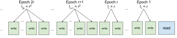
We will fixr=ω(1) wherer=O(logn) as the rate at which epochs will increase. In this section, we consider an epoch construction where epochs grow by the rate r everyr epochs. That is, the firstrepochs will each haverwrite operations. The next r epochs will each have r2 write operations, the next r epochs will each have r3 write operations and so forth. See Figure 4 for a diagram of this epoch construction. Once again, we define`ito be the size of thei-th epoch and si to be the total size of epochs 1, . . . , i. We note that

In other words, for epochi, there will be potentiallyrtimes more future opera-tions in comparison to the previous epoch construction of Section 3. On the other hand, we note that the number of epochs with at least max{√n, c2_{} write} op-erations is ˆk=Θ(rlog_r(n/(rc2))) =Θ(rlog_r(n/c)), which isΘ(r/logr) =ω(1) times larger than the number of epochs in the construction of Section 3. As a result, this epoch construction matches exactly the requirements that we wanted there to be more epochs which are required to be read by the read operation while only sacrificing that there are more futurewriteoperations for any epoch i. We now present a generalization of Lemma 3 which can be applied for the new epoch constructions that are introduced here and in Section 4.2.

Fig. 4: Diagram of epoch construction of Section 4.1.

Lemma 4. There exists an epoch i such that `i ≥ max{

√

n, c2_{} and both the}

following inequalities hold:

E[|T<i

w (Q)|] =O 

 

max e

X

j≥e se lj



· tw

ˆ k



andE[|T_ri(Q)|] =O(tr/k).ˆ

Proof. Using the same ideas of Lemma 3, we will show that there exists ˆk/2 + 1 epochs that satisfy the first statement and ˆk/2 + 1 epochs that satisfy the second statement. As a result, there exists at least one epoch satisfying both statements.

Pick an epochiuniformly at random from all ˆkepochs with at least max{√n, c2_}

write operations. Fix B1, . . . ,Bn−1 and Rarbitrarily. We will prove an upper bound on E[|T<i

before thepr-th operation, there are at mostsegood locations for thereadout of n/2 total locations. For any j ≥e, this cell probe has probability 2se/n of contributing toT<j

w (Q). Therefore, by linearity of expectation over the (n−1)tw expected cell probes:

E

_|T<i w (Q)|

`i = 1 ˆ k X

j:`j≥max{

√ n,c2_}

E

_|T<j w (Q)|

`j

≤ tw

ˆ k  max e X

j≥e 2se

`j 

.

Therefore, there exists ˆk/2 + 1 fixed epochsi such thatE[|T<i

w (Q)|/`i] over the choice of theread location is at most 3 times the above bound.

AsP iE[|T

i

r(Q)|]≤tr, there exists ˆk/2 + 1 epochsiwhere E[|Tri(Q)|]≤3tr completing the proof.

We can now plug the upper bounds of Lemma 4 into Lemma 2.

Theorem 3. Let DS be an (, δ)-differentially private RAM for n b-bit values implemented overw-bit cells. Assuming that =O(1)and0≤δ≤1/3,DShas failure probability at most 1/3 andw=Ω(log logn), then

tw=o((b/w) log(n/c)) =⇒ tr=ω((b/w) log(n/c)).

Proof. Recall we get the following inequality by applying convexity to the in-equality of Lemma 2 and noting thatc/`i=O(1) for our choicesi:

E[|T<i w (Q)|]

`i

w+ log twsi−1

E[|T<i w (Q)|]

+E[|Tri(Q)|]

w+ log tr

E[|Ti r(Q)|]

=Ω(b).

By applying Lemma 4, we get that E[|Ti

r(Q)|] = O(trlogr/(rlog(n/c))) and

E[|T<i

w (Q)|/`i] =O(twlogr/log(n/c)) since

_s j `j

+ sj `j+1

+. . .

≤2rX

j≥0 1

rj =O(r).

Plugging into the inequality above and assuming thatw=Ω(log logn),

tw+ (tr/r) =Ω((b/w) log(n/c)/logr) =⇒ tr=Ω((b/w) log(n/c)r/logr)

astw=o((b/w) log(n/c). Sincer/logr=ω(1), we complete the proof.

4.2 Second Epoch Construction

thereadoperation also cannot perform many cell probes into epochi, then each futurewriteoperation must encode a large amount of information about epoch i which will be used by the read operation. As a result, we can prove a large lower bound on tw. We now describe the epoch construction which enables us to prove such strong lower bounds ontw.

Fix ther=ω(1) wherer=O(logn) as the rate at which epochs will increase once again. This epoch construction will increase each epoch’s number ofwrite

operations by r. So, the first epoch will have r write operations, the second epoch will have r2write operations and so forth. In this case,

si−1=`i−1+`i−2+. . .≤ 1

r(`i+`i−1+. . .)≤2`i/r.

As a result, the number of future operations is Θ(1/r) times smaller than the epoch construction of Section 3. The number of epochs with at least max{√n, c2} writeoperations is ˆk=Θ(log_rn).

Theorem 4. Let DS be an (, δ)-differentially private RAM for n b-bit values implemented overw-bit cells. Assuming that =O(1)and0≤δ≤1/3,DShas failure probability at most 1/3 andw=Ω(log logn), then

tr=o((b/w) log(n/c)) =⇒ tw=ω((b/w) log(n/c)).

Proof. By applying Lemma 4, we get thatE[|Ti

r(Q)|] =O(trlogr/log(n/c)) and

E[|T<i

w (Q)|/`i] =O(twlogr/rlog(n/c)) since _s

j `j

+ sj `j+1

+. . .

≤2X

j≥0 1

rj =O(1).

Plugging into the inequality of Lemma 2 after applying convexity and noting that c/`i=O(1) and w=Ω(log logn),

(tw/r) +tr=Ω((b/w) log(n/c)/logr) =⇒ tw=Ω((b/w) log(n/c)r/logr)

sincetr=o((b/w) log(n/c)). Noting thatr/logr=ω(1) completes our proof.

5

Discussion

In this section, we discuss two extensions that follow from our lower bound techniques.

Larger Values of δ. In the proofs of Section 3 and 4, it is assumed thatδ≤1/3. Most practical scenarios require δmust be negligible in n, so the above results suffice. For theoretical exploration, we note that the proofs can be extended for any constantδ that is strictly smaller than 1. In particular, for any constantρ such thatδ < ρ < 1 and by picking a sufficiently large enough constantC, we can prove that Pr[Zi(Q(idx))≥b/C]≥ρwhich is a variation of Lemma 1 that suffices to prove a lower bound forδ.

6

Conclusion

In this work, we show that the Ω(log(n/c)) bandwidth overhead lower bound for the array maintenance problem with obliviousness extends to the weaker notion of differential privacy with reasonable privacy budgets of =O(1) and δ≤1/3. The result is surprising as differentially private RAM seems, at first, to provide significantly weaker privacy compared to the obliviousness guarantees of ORAM. Yet, differential privacy does not allow any asymptotic improvements in efficiency. This leads to the following natural open question: Does there exist a natural, weaker notion of privacy that enableso(log(n/c)) bandwidth overhead for the array maintenance problem?

References

1. E. Boyle, K.-M. Chung, and R. Pass. Oblivious parallel RAM and applications. In

Theory of Cryptography Conference, pages 175–204. Springer, 2016.

2. E. Boyle and M. Naor. Is there an oblivious RAM lower bound? InProceedings of the 2016 ACM Conference on Innovations in Theoretical Computer Science, pages 357–368. ACM, 2016.

3. D. Cash, P. Grubbs, J. Perry, and T. Ristenpart. Leakage-abuse attacks against searchable encryption. In Proceedings of the 22nd ACM SIGSAC conference on computer and communications security, pages 668–679. ACM, 2015.

4. T.-H. H. Chan, Y. Guo, W.-K. Lin, and E. Shi. Oblivious hashing revisited, and applications to asymptotically efficient ORAM and OPRAM. InInternational Conference on the Theory and Application of Cryptology and Information Security, pages 660–690. Springer, 2017.

5. B. Chen, H. Lin, and S. Tessaro. Oblivious parallel RAM: improved efficiency and generic constructions. InTheory of Cryptography Conference, pages 205–234. Springer, 2016.

6. K.-M. Chung, Z. Liu, and R. Pass. Statistically-secure ORAM with ˜O(log2n) overhead. InInternational Conference on the Theory and Application of Cryptology and Information Security, pages 62–81. Springer, 2014.

7. I. Damg˚ard, S. Meldgaard, and J. B. Nielsen. Perfectly secure oblivious RAM without random oracles. In Theory of Cryptography Conference, pages 144–163. Springer, 2011.